Recent research in generative models have borrowed ideas from classic probabilistic frameworks. Such a model is VAE, an improvement of variational inference. Similar to VI, VAE’s objective is to minimize the KL divergence between parameterized posterior and true posterior with respect to a variational family. Alternatively, a number of works attempt to enhance feature-learning and data-generating power of VAE by using different probability divergences. Among these approaches, Wasserstein distance brought from Optimal Transport (OT) is particularly promising. This article will survey several VI models that utilize Wasserstein distance.
Variational Inference
We first revisit VI whose idea is the base of VAE and its variants. Assume we have a set $ \small \mathbf{x} = \{ x_1, x_2, \dots, x_N \}$ contains $ \small N$ observations of data. VI aims to understand data by inferring low-dimensional representation from these (often high-dimensional) observations. To do so, it introduces a set of $ \small M$ latent variables $ \small \mathbf{z} = \{ z_1, z_2, \dots, z_M \} \sim q(\mathbf{z})$ with prior density $ \small q(\mathbf{z})$ and relates them to the observations through likelihood $ \small p(\mathbf{x} | \mathbf{z})$:
\[\small
\begin{align}
& p(\mathbf{z} | \mathbf{x}) = \frac{p(\mathbf{x}, \mathbf{z})}{p(\mathbf{x})} = \frac{p(\mathbf{x} | \mathbf{z}) q(\mathbf{z}) }{\int p(\mathbf{x}, \mathbf{z}) d \mathbf{z}} \label{eq1.1} \tag{1.1} \\
\text{where:} \: & p(\mathbf{z} | \mathbf{x}) \: \text{is posterior} \nonumber \\
& p(\mathbf{x}, \mathbf{z}) = p(\mathbf{x} | \mathbf{z}) q(\mathbf{z}) \: \text{is joint density of} \: \mathbf{x} \: \text{and} \: \mathbf{z} \nonumber \\
& p(\mathbf{x}) = \int p(\mathbf{x}, \mathbf{z}) d \mathbf{z} \: \text{is evidence, computed by marginalizing} \: \mathbf{z} \nonumber
\end{align}\]
The posterior represents distribution of latent variables given the observations, getting posterior is equivalent to learning data representation.
While $ \small p(\mathbf{x}, \mathbf{z})$ can be fully observable, the integral term is computationally expensive, thus the posterior is intractable
(Blei et al., 2017). VI overcomes this difficulty by approximating intractable posterior with simpler distribution. Specifically, it parameterizes prior $ \small q(\mathbf{z})$ with variational parameters $ \small \boldsymbol{\theta} = \{ \theta_1, \theta_2, …, \theta_M \} $ and then optimize them to achieve a good approximation of posterior in term of KL divergence.
Vanilla VI
To arrive with the optimization problem’s objective of VI, let’s consider:
\[\small
\begin{align}
& \log p(\mathbf{x}) = \log \int p(\mathbf{x} | \mathbf{z}) q_{\boldsymbol{\theta}} (\mathbf{z}) d\mathbf{z} = \log \mathbb{E}_{\mathbf{z} \sim q_{\boldsymbol{\theta}} (\mathbf{z})} [p(\mathbf{x} | \mathbf{z})] \label{eq1.2} \tag{1.2} \\
\text{where:} & \: q_{\boldsymbol{\theta}} (\mathbf{z}) \: \text{is parameterized prior} \nonumber
\end{align}\]
Since $ \small \log$ is concave function, by Jensen’s inequality:
\[\small
\begin{align}
\log \mathbb{E}_{ \mathbf{z} \sim q_{\boldsymbol{\theta}} (z)} [ p(\mathbf{x} | \mathbf{z})] \geq &\mathbb{E}_{\mathbf{z} \sim q_{\boldsymbol{\theta}}(\mathbf{z})} [ \log p(\mathbf{x} | \mathbf{z}) ] = \nonumber \\
&= \mathbb{E}_{q_{\boldsymbol{\theta}}(\mathbf{z})} \left[ \log \frac{ p(\mathbf{x}, \mathbf{z}) }{q_{\boldsymbol{\theta}}(\mathbf{z})} \right] = \nonumber \\
&= \mathbb{E}_{q_{\boldsymbol{\theta}}(\mathbf{z})} [ \log p(\mathbf{x}, \mathbf{z}) - \log q_{\boldsymbol{\theta}}(\mathbf{z}) ] = \mathcal{L}
\label{eq1.3} \tag{1.3}
\end{align}\]
The quantity $ \small \mathcal{L}$ is ELBO - Evidence Lower BOund.
We now show that the difference between $\ \small log p(x)$ and ELBO is exactly KL divergence between variational distribution, i.e. parameterized prior $ \small q_{\boldsymbol{\theta}}(\mathbf{z})$, and posterior:
\[\small
\begin{align}
\log p(\mathbf{x}) - \mathcal{L} &= \log p(\mathbf{x}) - \mathbb{E}_{q_{\boldsymbol{\theta}} (\mathbf{z})} [ \log p(\mathbf{x}, \mathbf{z}) - \log q_{\boldsymbol{\theta}}(\mathbf{z})] \nonumber \\
&= \mathbb{E}_{q_{\boldsymbol{\theta}} (\mathbf{z})} [\log p(\mathbf{x})] - \mathbb{E}_{q_{\boldsymbol{\theta}} (\mathbf{z})} [ \log p(\mathbf{x}, \mathbf{z}) - \log q_{\boldsymbol{\theta}} (\mathbf{z})] \nonumber \\
&= \mathbb{E}_{q_{\boldsymbol{\theta}} (\mathbf{z})} [\log p(\mathbf{x}) - \log p(\mathbf{x}, \mathbf{z}) + \log q_{\boldsymbol{\theta}}(\mathbf{z}) ] \nonumber \\
&= \mathbb{E}_{q_{\boldsymbol{\theta}} (\mathbf{z})} \left[ -\log \frac{p(\mathbf{x}, \mathbf{z})}{p(\mathbf{x})} + \log q_{\boldsymbol{\theta}}(\mathbf{z}) \right] \nonumber \\
&= \mathbb{E}_{q_{\boldsymbol{\theta}} (\mathbf{z})} \left[ \log q_{\boldsymbol{\theta}} (\mathbf{z}) - \log p(\mathbf{z} | \mathbf{x}) \right] \nonumber \\
&= \mathbb{E}_{q_{\boldsymbol{\theta}} (\mathbf{z})} \left[ \log \frac{q_{\boldsymbol{\theta}} (\mathbf{z})}{p(\mathbf{z} | \mathbf{x})} \right] = \text{KL}(q_{\boldsymbol{\theta}}(\mathbf{z}) \parallel p(\mathbf{z} | \mathbf{x})) \label{eq1.4} \tag{1.4} \\
\text{where:} \: \text{KL} (q \parallel p ) \: &\text{is Kullback-Leibler divergence between} \: q \: \text{and} \: p \nonumber
\end{align}\]
Another way to express ($\ref{eq1.4}$) is:
\[\small
\begin{align}
\log p(\mathbf{x}) &= \mathbb{E}_{ \mathbf{z} \sim q_{\boldsymbol{\theta}}(\mathbf{z}) } \left[ \log p(\mathbf{x}) \right] \nonumber \\
&= \mathbb{E}_{ \mathbf{z} \sim q_{\boldsymbol{\theta}}(\mathbf{z}) } \left[ \log \frac{p(\mathbf{x} | \mathbf{z}) q_{\boldsymbol{\theta}}(\mathbf{z}) }{p(\mathbf{z} | \mathbf{x})} \right] \nonumber \\
&= \mathbb{E}_{q_{\boldsymbol{\theta}} (\mathbf{z})} \left[ \log \frac{q_{\boldsymbol{\theta}}(\mathbf{z} | \mathbf{x}) p(\mathbf{x} | \mathbf{z}) p(\mathbf{z})}{q_{\boldsymbol{\theta}}(\mathbf{z} | \mathbf{x}) p(\mathbf{z} | \mathbf{x}) } \right] \nonumber \\
&= \mathbb{E}_{q_{\boldsymbol{\theta}} (\mathbf{z})} \left[ \log \frac{q_{\boldsymbol{\theta}}(\mathbf{z} | \mathbf{x})}{p (\mathbf{z} | \mathbf{x})} + \log p(\mathbf{x} | \mathbf{z}) - \log \frac{q_{\boldsymbol{\theta}}(\mathbf{z} | \mathbf{x})}{p(\mathbf{z})} \right] \nonumber \\
&= \mathbb{E}_{q_{\boldsymbol{\theta}}(\mathbf{z})} \left[ \log \frac{q_{\boldsymbol{\theta}}(\mathbf{z} | \mathbf{x})}{p(\mathbf{z} | \mathbf{x})} \right] + \mathbb{E}_{q_{\boldsymbol{\theta}}(\mathbf{z})} \left[ \log p(\mathbf{x} | \mathbf{z}) \right] - \mathbb{E}_{q_{\boldsymbol{\theta}}(\mathbf{z})} \left[ \log \frac{q_{\boldsymbol{\theta}}(\mathbf{z} | \mathbf{x})}{p(\mathbf{z})} \right] \nonumber \\
&= \text{KL} \left( q_{\boldsymbol{\theta}}(\mathbf{z} | \mathbf{x}) \parallel p(\mathbf{z} | \mathbf{x}) \right) + \mathbb{E}_{q_{\boldsymbol{\theta}}(\mathbf{z})} \left[ \log p(\mathbf{x} | \mathbf{z}) \right] - \text{KL} \left( q_{\boldsymbol{\theta}}(\mathbf{z} | \mathbf{x}) \parallel p(\mathbf{z}) \right) \nonumber
\end{align}\]
So:
\[\small
\begin{align}
\implies \: & \log p(\mathbf{x}) - \text{KL} \left( q_{\boldsymbol{\theta}}(\mathbf{z} | \mathbf{x}) \parallel p(\mathbf{z} | \mathbf{x}) \right) = \mathbb{E}_{q_{\boldsymbol{\theta}}(\mathbf{z})} \left[ \log p(\mathbf{x} | \mathbf{z}) \right] - \text{KL} \left( q_{\boldsymbol{\theta}}(\mathbf{z} | \mathbf{x}) \parallel p(\mathbf{z}) \right) \label{eq1.4a} \tag{1.4a} \\
& \text{where:} \: p(\mathbf{z}) \: \text{is true distribution of} \: \mathbf{z} \nonumber
\end{align}\]
From ($\ref{eq1.4}$), the posterior $ \small p(\mathbf{z} | \mathbf{x})$ can be approximated by $ \small q_{\boldsymbol{\theta}}(\mathbf{z})$ as long as we can find a parameters set $ \small \boldsymbol{\theta}$ to have $ \small \text{KL}(q_{\boldsymbol{\theta}}(\mathbf{z}) \parallel p(\mathbf{z} | \mathbf{x})) = 0$. Although fulfilling that requirement is practically impossible, we could still reach the KL divergence’s minima. Hence, VI simply turns computing task of intractable posterior into optimization problem with following objective:
\[\small
\begin{align*}
\underset{\boldsymbol{\theta}}{\min} \: \text{KL}(q_{\boldsymbol{\theta}}(\mathbf{z}) \parallel p(\mathbf{z} | \mathbf{x}))
\end{align*}\]
Note that $ \small \log p(\mathbf{x})$ is a constant quantity w.r.t $ \small \boldsymbol{\theta}$, to minimize $ \small \text{KL}(q_{\boldsymbol{\theta}}(\mathbf{z}) \parallel p(\mathbf{z} | \mathbf{x}))$ is equivalent to maximize the ELBO. One way of computing ELBO analytically is to restrict models to conjugate exponential family distribution. But we will focus on other approaches which are related to VAE.
Mean-Field VI (MFVI)
Choosing prior distribution leads to a trade-off between complexity and quality of posterior. We want an approximation that can express prior well yet must be simple enough to make itself tractable. A common choice is mean-field approximation, an adaption of mean-field theory in physics. Under mean-field assumption, MFVI factorizes $ \small q_{\boldsymbol{\theta}}(\mathbf{z})$ into $ \small M$ factors where each factor is governed by its own parameter and is independent of others:
\[\small
\begin{align}
q_{\boldsymbol{\theta}}(\mathbf{z}) = \prod_{j=1}^{M} q_{\theta_j}(z_j) \label{eq1.5} \tag{1.5}
\end{align}\]
Remember that mean-field approximation does not concern the correlation between latent variables, it becomes less accurate when true posterior variables are highly dependent.
For brevity, we shorten $ \small q_{\theta_j}(z_j)$ to $ \small q(z_j)$ and denote $ \small \mathbf{z}_{-j} = \mathbf{z} \setminus {z_j}$ as the latent set excluding variable $ \small z_j $.
By the assumption, we have:
\[\small
\begin{align}
p(\mathbf{x}, \mathbf{z}) &= p(z_j, \mathbf{x} | z_{-j}) q(\mathbf{z}_{-j}) \nonumber \\
&= p(z_j, \mathbf{x} | z_{-j}) \prod_{i \neq j} q(z_i) \label{eq1.6} \tag{1.6} \\
\mathbb{E}_{q(\mathbf{z})} \left[ \log q (\mathbf{z}) \right] &= \sum_{j=1}^{M} \mathbb{E}_{q(z_j)} \left[ \log q(z_j) \right] \label{eq1.7} \tag{1.7}
\end{align}\]
Hence:
\[\small
\begin{align}
\mathcal{L} &= \int_{\mathbf{z}} \left( \prod_{i=1}^{M} q_i (z_i) \right) \log \frac{p(\mathbf{x}, \mathbf{z})} {\prod_{k=1}^{M} q_k(z_k) } d \mathbf{z} \nonumber \\
&= \int_{\mathbf{z}} \left( \prod_{i=1}^{M} q_i (z_i) \right) \left( \log p(\mathbf{x}, \mathbf{z}) - \sum_{k=1}^{M} \log q_k(z_k) \right) d \mathbf{z} \nonumber \\
&= \int_{z_j} q(z_j) \int_{\mathbf{z}_{-j }} \left( \prod_{i \neq j} q_i(z_i) \right) \left[ \log p(\mathbf{x}, \mathbf{z}) - \sum_{k=1}^{M} \log q_k(z_k) \right) d \mathbf{z} \nonumber \\
&= \int_{z_j} q(z_j) \int_{\mathbf{z}_{-j }} \left( \prod_{i \neq j} q_i(z_i) \right) \log p(\mathbf{x}, \mathbf{z}) d \mathbf{z} \nonumber \\
& - \int_{z_j} q(z_j) \int_{\mathbf{z}_{-j }} \left( \prod_{i \neq j} q_i(z_i) \right) \sum_{k=1}^{M} \log q_k(z_k) d \mathbf{z} \label{eq1.8} \tag{1.8}
\end{align}\]
Here we substitute $ \small \int_{\mathbf{z}} d \mathbf{z}$ for $ \small \int_{z_1} \int_{z_2} \dots \int_{z_M} d z_1 d z_2 \dots d z_M$.
On the other hand:
\[\small
\begin{align}
\int_{\mathbf{z}_{-j }} \left( \prod_{i \neq j} q_i(z_i) \right) \log p(\mathbf{x}, \mathbf{z}) dz_1 \dots dz_{j-1} dz_{j+1} \dots dz_M = \mathbb{E}_{q(\mathbf{z}_{-j})} \log p(\mathbf{x}, \mathbf{z}) \label{eq1.9} \tag{1.9}
\end{align}\]
From ($\ref{eq1.8}$) and ($\ref{eq1.9}$):
\[\small
\begin{align}
\mathcal{L} &= \int_{z_j} q(z_j) \mathbb{E}_{q(\mathbf{z}_{-j})}[ \log p(\mathbf{x}, \mathbf{z}) ] dz_j - \int_{z_j} q(z_j) \int_{\mathbf{z}_{-j }} \left( \prod_{i \neq j} q_i(z_i) \right) \sum_{k=1}^{M} \log q_k(z_k) d z_1 d z_2 \dots d z_M \nonumber \\
&= \int_{z_j} q(z_j) \mathbb{E}_{q(\mathbf{z}_{-j})}[ \log p(\mathbf{x}, \mathbf{z}) ] dz_j
- \int_{z_j} q(z_j) \log q(z_j) \underbrace{\int_{\mathbf{z}_{-j}} \left( \prod_{i \neq j}q_i(z_i) \right) dz_1 \dots dz_M }_{=1} \nonumber \\
&- \underbrace{\int_{z_j} q(z_j) dz_j }_{=1} \int_{\mathbf{z}_{-j}} \left( \prod_{i \neq j} q_i(z_i) \right) \sum_{k \neq j} \log q_k (z_k) dz_1 \dots dz_{j-1} dz_{j+1} \dots dz_M \nonumber \\
&= \int_{z_j} q(z_j) \mathbb{E}_{q(\mathbf{z}_{-j})}[ \log p(\mathbf{x}, \mathbf{z}) ] dz_j - \int_{z_j} q(z_j) \log q(z_j) dz_j \nonumber \\
&- \int_{\mathbf{z}_{-j}} \left( \prod_{i \neq j} q_i(z_i) \right) \sum_{k \neq j} \log q_k(z_k) dz_1 \dots dz_{j-1} dz_{j+1} \dots dz_M \nonumber \\
&= \int_{z_j} q(z_j) \left( \mathbb{E}_{q(\mathbf{z}_{-j})}[ \log p(\mathbf{x}, \mathbf{z}) ] - \log q(z_j) \right) dz_j + C_{-j} \label{eq1.10} \tag{1.10} \\
\text{where:} \: & C_{-j} \: \text{contains all constant quantities w.r.t} \: z_j \nonumber
\end{align}\]
Using ($\ref{eq1.6}$), we can come up with another form:
\[\small
\begin{align}
\mathcal{L} &= \int_{\mathbf{z}_j} q(z_j) \left( \mathbb{E}_{q(\mathbf{z}_{-j})}[ \log p(z_j, \mathbf{x} | \mathbf{z}_{-j}) + \log q(\mathbf{z}_{-j})] - \log q(z_j) \right) dz_j + C_{-j} \nonumber \\
&= \int_{z_j} q(z_j) \left( \mathbb{E}_{q(\mathbf{z}_{-j})}[\log p(z_j, \mathbf{x} | \mathbf{z}_{-j})] - \log q(z_j) \right) dz_j \nonumber \\
&+ \left( \int_{z_j} q(z_j) dz_j \right) \mathbb{E}_{q(\mathbf{z}_{-j})} [\log q(\mathbf{z}_{-j})] + C_{-j} \nonumber \\
&= \int_{z_j} q(z_j) \left( \mathbb{E}_{q(\mathbf{z}_{-j})}[\log p(z_j, \mathbf{x} | \mathbf{z}_{-j})] - \log q(z_j) \right) dz_j + C_{-j}^{\prime} \label{eq1.11} \tag{1.11}
\end{align}\]
Our objective now becomes:
\[\small
\begin{align}
& \underset{q(z_j)}{\max} \int_{z_j} q(z_j) \left( \mathbb{E}_{q(\mathbf{z}_{-j})}[ \log p(z_j, \mathbf{x} | \mathbf{z}_{-j}) ] - \log q(z_j) \right) dz_j + C_{-j}^{\prime} \label{eq1.12} \tag{1.12} \\
\text{s.t.:} & \: \int_{z_j}q(z_j)dz_j = 1, \: \forall j \in \{1,2,\dots,M \} \nonumber
\end{align}\]
Problem ($\ref{eq1.12}$) can be easily solved by Lagrange multiplier:
\[\small
\begin{align}
\max &\: \mathcal{L} - \sum_{j=1}^{M} \lambda_j \int_{z_j}q(z_j)dz_j \label{eq1.13} \tag{1.13}
\end{align}\]
Taking derivative of ($\ref{eq1.13}$) w.r.t $ \small q(z_j)$:
\[\small
\begin{align}
\frac{\partial \mathcal{L}}{\partial q(z_j)} &= \frac{\partial}{\partial q(z_j)} \left[ q(z_j)
\left( \mathbb{E}_{q(\mathbf{z}_{-j})} [\log p(z_j, \mathbf{x} | \mathbf{z}_{-j} ) -\log q(z_j) ] \right) - \lambda_j q(z_j) \right] \nonumber \\
&= \mathbb{E}_{q(\mathbf{z}_{-j})}[\log p(z_j, \mathbf{x} | \mathbf{z}_{-j}) ] - \log q(z_j) - 1 - \lambda_j \label{eq1.14} \tag{1.14}
\end{align}\]
Set the partial derivative to $ \small 0$ to get the updating form of $ \small q(z_j)$:
\[\small
\begin{alignat}{2}
& \log q(z_j) &&= \mathbb{E}_{q(\mathbf{z}_{-j})}[\log p(z_j, \mathbf{x} | \mathbf{z}_{-j} )] - 1 - \lambda_j \nonumber \\
& &&= \mathbb{E}_{q(\mathbf{z}_{-j})}[\log p(z_j, \mathbf{x} | \mathbf{z}_{-j} )] + const \nonumber \\
\implies & q(z_j) &&= \frac{\exp \left\{ \mathbb{E}_{q(\mathbf{z}_{-j})}[\log p(z_j, \mathbf{x} | \mathbf{z}_{-j} )] \right\} }{Z_j} \nonumber \\
\implies & q(z_j) && \propto \exp \left\{ \mathbb{E}_{q(\mathbf{z}_{-j})}[\log p(z_j, \mathbf{x} | \mathbf{z}_{-j} )] \right\} \nonumber \\
& && \propto \exp \left\{ \mathbb{E}_{q(\mathbf{z}_{-j})}[\log p(\mathbf{x}, \mathbf{z})] \right\} \label{eq1.15} \tag{1.15} \\
& \text{where:} \: && Z_j \: \text{is a normalization constant} \nonumber
\end{alignat}\]
Since $ \small q(z_j)$ and $ \small q(z_i)$ are independent for any $ \small j \neq i, : i, j \in {1, 2, \dots, M }$, maximizing EBLO w.r.t $ \small \boldsymbol{\theta}$ can be done by alternately maximizing ELBO w.r.t $ \small \theta_j$ for $ \small j=1,2,\dots,M$. Therefore, under mean-field approximation, maximum of ELBO can be accomplished by iteratively updating variational distribution of each latent variable by rule ($\ref{eq1.15}$) until convergence. This algorithm’s called coordinate ascent.
Stochastic VI (SVI)
Various VI models are not feasible for big datasets, for instance, MFVI’s updating rule ($\ref{eq1.15}$) is exhausted for huge number of observations since it must process every single data point. Different from these approaches, SVI employs stochastic optimization for efficiently optimizing its objective under big data circumstance.
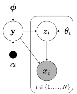
Fig1.1: Graphical model of SVI: observations $x_i$, local underlying variables $z_i$s, global latent variable $\mathbf{y}$, local variational parameter $\theta_i$, global variational parameter $\boldsymbol{\phi}$, hyper-parameter $\alpha$. Dashed line indicate variational approximation.
Instead of only considering local (i.e. per data point) latent variable $ \small z_i$ and their corresponding variational parameter $ \small \theta_i$, SVI introduces global latent variable $ \small \mathbf{y}$ and global variational parameter $ \small \boldsymbol{\phi}$. In detail, we have $ \small \{ z_i \text{s}, \mathbf{y} \} $ as latent variables and $ \small { \theta_i, \boldsymbol{\phi} } $ as variational parameter for $ \small i = 1, 2, \dots, N$ (recall that $ \small N$ is number of observations). Furthermore, we assume the model depends on a hyper-paremeter $ \small \alpha$. Unlike vanilla VI, SVI’s objective is summed over contributions of all $ \small N$ individual data points. This setting allows stochastic optimization work. Later we will learn that VAE also adopts it.
Variational distribution follows below assumption:
\[\small
\begin{align}
& q(\mathbf{z}, \mathbf{y}) = q_{\boldsymbol{\phi}}(\mathbf{y}) \prod_{i=1}^{N} q_{\theta_i}(z_i) = q(\mathbf{y}) \prod_{i=1}^{N} q(z_i)
\label{eq1.16} \tag{1.16} \\
\text{where:} & \: q(\mathbf{y}), \: q(z_i) \: \text{are abbreviation of} \: q_{\boldsymbol{\phi}}(\mathbf{y}), \: q_{\theta_i}(z_i) \: \text{respectively} \nonumber
\end{align}\]
Joint distribution is factorization of global term and local terms:
\[\small
\begin{align}
p(\mathbf{x}, \mathbf{z}, \mathbf{y} \mid \alpha) &= p(\mathbf{y} \mid \alpha) \prod_{i=1}^{N} p(x_i, z_i \mid \mathbf{y}, \alpha)
\label{eq1.17} \tag{1.17} \\
p(x_i, z_i \mid \mathbf{y}, \alpha) &= p(x_i \mid z_i, \mathbf{y}, \alpha) p(z_i \mid \mathbf{y}, \alpha) \label{eq1.18} \tag{1.17}
\end{align}\]
SVI’s objective then becomes:
\[\small
\begin{align}
\mathcal{L} &= \mathbb{E}_{q(\mathbf{z}, \mathbf{y})} \left[\log \frac{p(\mathbf{x}, \mathbf{z}, \mathbf{y} \mid \alpha)}{q(\mathbf{z}, \mathbf{y})} \right] \nonumber \\
&= \mathbb{E}_q \left[ \log p(\mathbf{x}, \mathbf{z}, \mathbf{y} \mid \alpha) \right] - \mathbb{E}_q \left[ \log q(\mathbf{z}, \mathbf{y}) \right] \tag*{($\mathbb{E}_q$ is abbreviation of $\mathbb{E}_{q(\mathbf{z}, \mathbf{y})}$ )} \nonumber \\
&= \mathbb{E}_q \left[ \log \left( p(\mathbf{y} \mid \alpha) \prod_{i=1}^{N} p(x_i, z_i \mid \mathbf{y}, \alpha) \right) \right] - \mathbb{E}_q \left[ \log \left( q(\mathbf{y}) \prod_{i=1}^{N} q(z_i) \right) \right] \nonumber \\
&= \mathbb{E}_q \left[ \log p(\mathbf{y} \mid \alpha) \right] + \sum_{i=1}^{N} \mathbb{E}_q \left[ \log p(x_i, z_i \mid \mathbf{y}, \alpha) \right] - \mathbb{E}_q \left[ \log q(\mathbf{y}) \right] - \sum_{i=1}^{N} \mathbb{E}_q \left[ \log q(z_i) \right] \nonumber \\
&= \mathbb{E}_q \left[ \log p(\mathbf{y} \mid \alpha) - \log q(\mathbf{y}) \right] + \sum_{i=1}^{N} \left[ \log p(x_i, z_i \mid \mathbf{y}, \alpha) - \log q(z_i) \right] \nonumber \\
&= \mathbb{E}_q \left[ \log p(\mathbf{y} \mid \alpha) - \log q(\mathbf{y}) \right] + \sum_{i=1}^{N} \left[ \log p(x_i \mid z_i, \mathbf{y}, \alpha) + \log p(z_i \mid \mathbf{y}, \alpha) - \log q(z_i) \right] \label{eq1.19} \tag{1.19}
\end{align}\]
Though coordinate ascent can optimize function ($\ref{eq1.19}$), stochastic gradient descent should be more efficient. Particularly, in each iteration, random-selected mini-batches of size $S$ are used to obtain stochastic estimate $ \small \hat{\mathcal{L}}$ of ELBO:
\[\small
\begin{align}
\hat{\mathcal{L}} &= \mathbb{E}_q \left[ \log p(\mathbf{y} \mid \alpha) - \log q(\mathbf{y}) \right] + \frac{N}{S} \sum_{i=1}^{S} \left[ \log p(x_{i_s} \mid z_{i_s}, \mathbf{y}, \alpha) + \log p(z_{i_s} \mid \mathbf{y}, \alpha) - \log q(z_{i_s}) \right] \label{eq1.20} \tag{1.20}
\end{align}\]
$ \small i_s$s are indices of mini-batch that must be uniformly drawn at random. $ \small S$ is often chosen such that $ \small 1 \leq S \ll N$.
Computation cost on small batch-size $ \small S$ is less expensive than on entire dataset. A noisy estimator of gradient of ELBO then can be achieved via $ \small \hat{\mathcal{L}}$. As a result, optimal of the objective function can be acquired using stochastic gradient optimization. Several important results of SVI models have been published, one may refer to (Hensman et al., 2012), (Khan et al., 2018, Hoffman et al., 2013) for more details.
Lastly, there is a trade-off between computation’s efficiency and gradient estimator’s variance. Large batch-size $ \small S$ which consumes more computational resource reduces variance of gradient estimate. In this case, less noisy gradient allows us to have larger learning rate, thus it’s faster to reach the convergence state and also more favored for global parameters to perform inference. On the other hand, small mini-batches relaxes the cost of iterating over local parameters. Various methods have been proposed to address this problem, notably can include adaptive learning rate and mini-batch size and variance reduction. It’s worth to mention that alongside stochastic VI, there exists other interesting approaches to speed up convergence process such as Collapsed, Sparse, and Distributed VI. All of them leverage the structure of certain models to attain the goal (Zhang et al., 2017).