Variational Auto-encoders (VAE)
VAE is another scale-up variant of VI. It employs deep neural networks to perform large datasets of high-dimensional samples such as images. Apart from representation learning, VAE is more advanced than VI at ability of reconstructing high quality samples.
Amortized Variational Inference
In VI models, each local variable is governed by its own variational parameter, e.g. in SVI, parameter $ \small \theta_i$ corresponds to latent variable $ \small z_i$. To maximize ELBO, we have to optimize objective function w.r.t all variational parameters. Consequently, the larger number of parameters is, the more expensive computational cost is.
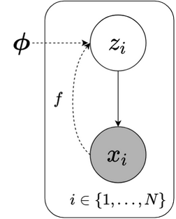
Fig2.1: Graphical model of Amortized VI. Dashed line indicates variational approximation.
Amortized VI reforms SVI structure to lower the cost. In particular, it assumes that optimal $ \small z_i$’s can be represented as a function of $ \small x_i$s, $ \small z_i = f(x_i)$, i.e. $ \small z_i$s are features of $ \small x_i$s. Of course, local variational parameters are removed. Employing a function whose parameters are shared across all data points allows past computation to support future computation. Once the function is estimated (say, after few optimization steps), local variables obviously can be computed by passing new data points to $ \small f(\cdot)$. This is why we name it amortized. Function $ \small f(\cdot)$ implements a deep neural network called inference network to make a powerful predictor.
Reparameterization and Monte Carlo
Reparameterization trick and Monte Carlo method are necessary for VAE to work. One challenge in VAE, and gradient-based models in general, is to compute gradient of expectation of a smooth function. A common way to achieve such gradient without analytical methods is to reparameterize variable first, then estimate gradient by Monte Carlo sampling. The former step serves two purposes, one for back-propagation’s, one for reducing complexity of the latter step. (Feel free to skip this section if you are already familiar with those concepts.)
Let’s estimate the following gradient which later shows up in VAE:
\[\small
\begin{align}
\nabla_{\theta} \mathbb{E}_{q_{\theta}(z)} \left[ f(z) \right] = \nabla_{\theta} \int q_{\theta}(z)f(z)dz \label{eq2.1} \tag{2.1}
\end{align}\]
The naive Monte Carlo gradient estimator of ($\ref{eq2.1}$) is:
\[\small
\begin{align*}
\nabla_{\theta} \mathbb{E}_{q_{\theta}(z)} \left[ f(z) \right] &= \mathbb{E}_{q_{\theta}(z)} \left[ f(z) \nabla_{q_{\theta}(z)} \log q_{\theta}(z) \right] \approx \frac{1}{L} \sum_{i=1}^{L} f(z) \nabla_{q_{\theta}(z_i)} \log q_{\theta}(z_i) \\
\text{where:} \: & L \: \text{is number of samples} \nonumber \\
& z_i \sim q_{\theta}(z)
\end{align*}\]
This often results in very high variance estimate and impractical (Blei et al., 2012). Fortunately, reparameterization trick can resolve the problem.
The idea of reparameterization is to transform one distribution into another form by additive/multiplicative location-scale transformations, these are basically co-ordinate transformations. This way, we can express diverse and flexible class of distributions in combination of multiple simpler terms.
We illustrate normal distribution case since it is widely used in machine learning and also appears in VAE. Given variable $ \small z$ drawn from normal distribution and standard Gaussian noise $ \small \varepsilon$, $ \small z$ can be reparameterized by following transformation:
\[\small
\begin{align}
& z = \mu + \varepsilon \sigma \label{eq2.2} \tag{2.2} \\
\text{where:} \: & z \sim \mathcal{N}(z ; \mu, \sigma^2) \nonumber \\
& \varepsilon \sim \mathcal{N}(\varepsilon ; 0, 1) \nonumber
\end{align}\]
With the transformation from distribution $ \small q(\epsilon)$ to $ \small q_{\theta}(z)$, the probability contained in a differential area must be invariant under change of variables, i.e. $ \small {\lvert} {q_{\theta}(z)dz} {\rvert} = {\lvert} {q(\varepsilon) d \varepsilon} {\rvert} $. Together with ($\ref{eq2.1}$), we have:
\[\small
\begin{alignat}{2}
& \nabla_{\theta} \mathbb{E}_{q_{\theta}(z)} \left[ f(z) \right] &&= \: \nabla_{\theta} \int q_{\theta}(z)f(z)dz \nonumber \\
=& \: \nabla_{\theta} \int q(\varepsilon) f(z) d \varepsilon &&= \: \nabla_{\theta} \int q(\varepsilon) f(g(\varepsilon, \theta)) d \varepsilon \nonumber \\
=& \: \nabla_{\theta} \mathbb{E}_{q(\varepsilon)} \left[ f(g(\varepsilon, \theta)) \right] &&= \: \mathbb{E}_{q(\varepsilon)} \left[ \nabla_{\theta} f(g(\varepsilon, \theta)) \right] \label{eq2.3} \tag{2.3}
\end{alignat}\]
Here $ \small \theta$ is the set of parameters and $g(\varepsilon, \theta)$ is the transformation. $ \small q_{\theta}(z)$ and $ \small q(\varepsilon)$ are density functions of distribution of $ \small z$ and $ \small \varepsilon$ respectively. For instance, when $ \small z$ has normal distribution, $ \small \theta$ would be $ \small {\mu, \sigma }$ and $ \small g(\varepsilon, \theta)$ would be equation ($\ref{eq2.2}$).
Gradient in ($\ref{eq2.3}$) now can be acquired using Monte Carlo estimation. Monte Carlo method allows us to estimate result of certain tasks by performing deterministic computation on large number of inputs that are sampled from a probability distribution on pre-defined domain. It eases the worry of analytically computing intractable quantity. For integral task, it is simple and straightforward:
\[\small
\begin{align}
\mathbb{E}_{q(z)} \left[ f(z) \right] &= \int f(z) q(z) dz \approx \frac{1}{L} \sum_{l=1}^{L} f(z_l) \label{eq2.4} \tag{2.4} \\
\text{where:} \: & z_l \sim q(z) \: \text{for} \: l=1,2,\dots,L \nonumber
\end{align}\]
The larger number of samples is, the more accurate estimation is.
From ($\ref{eq2.3}$) and ($\ref{eq2.4}$):
\[\small
\begin{align}
& \mathbb{E}_{q_{\theta}(z)} \left[ f(z) \right] \approx \frac{1}{L} \sum_{i=1}^{L} f(g(\varepsilon_l, \theta)) \nonumber \\
& \nabla_{\theta} \mathbb{E}_{q_{\theta}(z)} \left[ f(z) \right] = \mathbb{E}_{q(\varepsilon)} \left[ \nabla_{\theta} f(g(\varepsilon, \theta)) \right] \approx \frac{1}{L} \sum_{l=1}^{L} \left[ \nabla_{\theta} f(g(\varepsilon_l, \theta)) \right] \label{eq2.5} \tag{2.5} \\
& \text{where:} \: \varepsilon_l \sim q(\varepsilon) \nonumber
\end{align}\]
Sampling $ \small \varepsilon$ clearly is easier than sampling $ \small z$ directly, the problem ($\ref{eq2.1}$) turns out to be feasible.
VAE adopts SVI and Amortized VI to make a powerful generative model. The term “generative” bases on the fact that VAE employs a neural network as generative network alongside mentioned inference network.
For simplicity, we only study VAE in setting of deep latent Gaussian model, i.e. hidden variable $ \small z$ has (parameterized) normal distribution. Other settings which are less common can be found at (Kingma’s Thesis, 2017), (Kingma and Welling, 2014).
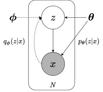 fig2.2a Grapical model
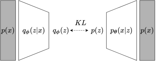 fig 2.2b Neural networks
Fig2.2 (a) Fig 2.2a shows probabilistic VAE model. Dashed lines indicate variational approximation, solid lines present generative model. $\boldsymbol{\phi}$ is parameters of variational distribution $q_{\boldsymbol{\phi}}(z \| x)$. $\boldsymbol{\theta}$ is parameter of generative model $p(z) p_{\boldsymbol{\theta}}(x \| z) $. (b) Fig 2.2b presents VAE deep learning model. $q_{\boldsymbol{\phi}}(z \| x)$ and $p_{\boldsymbol{\theta}}(x \| z)$ are replaced by neural networks.
Figure 2.2 demonstrates VAE in two perspectives: (a) graphical model and (b) deep learning model. Inference model with variational distribution $ \small q_{\boldsymbol{\phi}}(z | x)$ and generative model $ \small p(z) p_{\boldsymbol{\theta}}(x | z)$ are performed by encoder network and decoder network respectively. The variational parameters $ \small \boldsymbol{\phi}$ and generative model’s parameters $ \small \boldsymbol{\theta} $ are simultaneously optimized. While VI considers a set of data points and a set of latent variables (part 1), VAE can take a single data point as input thanks to amortized setting.
Similar to eq1.4 or eq1.4a, we can come up with objective function of VAE. Recall that out data points are i.i.d, the marginal log-likelihood is $ \small \log p(\mathbf{x}) = \sum_{i=1}^{N} \log p(x_i)$. Therefore, we only concern about a single observation:
\[\small
\begin{align}
\log p(x) &= \mathbb{E}_{z \sim q_{\boldsymbol{\phi}} (z|x)} \left[ \log p(x) \right] \nonumber \\
&= \mathbb{E}_{q_{\boldsymbol{\phi}} (z|x)} \left[ \log \frac{p_{\boldsymbol{\theta}}(x, z)}{p(z|x)} \right] \nonumber \\
&= \mathbb{E}_{q_{\boldsymbol{\phi}} (z|x)} \left[ \log \frac{p_{\boldsymbol{\theta}}(x, z) q_{\boldsymbol{\phi}}(z|x) }{p(z|x) q_{\boldsymbol{\phi}}(z|x)} \right] \nonumber \\
&= \mathbb{E}_{q_{\boldsymbol{\phi}} (z|x)} \left[ \frac{q_{\boldsymbol{\phi}}(z|x) }{p(z|x) } \right] + \mathbb{E}_{q_{\boldsymbol{\phi}} (z|x)} \left[ \log p_{\boldsymbol{\theta}}(x, z) - \log q_{\boldsymbol{\phi}}(z|x) \right] \nonumber \\
&= \text{KL} \left( q_{\boldsymbol{\phi}}(z|x) \parallel p(z|x) \right) + \mathbb{E}_{q_{\boldsymbol{\phi}} (z|x)} \left[ \log p_{\boldsymbol{\theta}}(x, z) - \log q_{\boldsymbol{\phi}}(z|x) \right] \nonumber \\
&= \text{KL} \left( q_{\boldsymbol{\phi}}(z|x) \parallel p(z|x) \right) + \mathbb{E}_{q_{\boldsymbol{\phi}} (z|x)} \left[ \log p_{\boldsymbol{\theta}}(x| z) + \log p(z) - \log q_{\boldsymbol{\phi}}(z|x) \right] \nonumber \\
&= \text{KL} \left( q_{\boldsymbol{\phi}}(z|x) \parallel p(z|x) \right) + \mathbb{E}_{q_{\boldsymbol{\phi}} (z|x)} \left[ \log p_{\boldsymbol{\theta}}(x|z) \right] - \text{KL}\left( q_{\boldsymbol{\phi}}(z|x) \parallel p(z) \right) \label{eq2.6} \tag{2.6}
\end{align}\]
\[\small
\begin{align}
\implies \log p(x) - \text{KL} \left( q_{\boldsymbol{\phi}}(z|x) \parallel p(z|x) \right) &= \underbrace{ -\text{KL}\left( q_{\boldsymbol{\phi}}(z|x) \parallel p(z) \right) + \mathbb{E}_{q_{\boldsymbol{\phi}} (z|x)} \left[ \log p_{\boldsymbol{\theta}}(x|z) \right] }_{\ell} \label{eq2.6a} \tag{2.6a}
\end{align}\]
Minimizing KL divergence between variational posterior and true posterior equivalents to maximizing ELBO $ \small \ell$. The variational lower bound of a single data point $ \small x_i$:
\[\small
\begin{align}
\ell_i (\boldsymbol{\phi}, \boldsymbol{\theta}) = - \text{KL}\left( q_{\boldsymbol{\phi}}(z|x_i) \parallel p(z) \right) + \mathbb{E}_{q_{\boldsymbol{\phi}} (z|x_i)} \left[ \log p_{\boldsymbol{\theta}}(x_i|z) \right] \label{eq2.7} \tag{2.7}
\end{align}\]
The objective function on entire data set should be:
\[\small
\begin{align}
\mathcal{L} &= \sum_{i=1}^{N} \ell_i (\boldsymbol{\phi}, \boldsymbol{\theta}) = - \sum_{i=1}^{N} \text{KL} \left( q_{\boldsymbol{\phi}}(z|x_i) \parallel p(z) \right) + \sum_{i=1}^{N} \mathbb{E}_{q_{\boldsymbol{\phi}} (z|x_i)} \left[ \log p_{\boldsymbol{\theta}} (x_i | z) \right] \nonumber \\
&= \mathbb{E}_{x \sim p(x)} \left[ - \text{KL}\left( q_{\boldsymbol{\phi}}(z|x) \parallel p(z) \right) \right] + \mathbb{E}_{x \sim p(x)} \left[ \mathbb{E}_{q_{\boldsymbol{\phi}} (z|x)} \left[ \log p_{\boldsymbol{\theta}} (x | z) \right] \right] \label{eq2.8} \tag{2.8}
\end{align}\]
The quantity $ \small \text{KL}\left( q_{\boldsymbol{\phi}}(z|x_i) \parallel p(z) \right) $ can be integrated analytically under certain assumption. Let’s consider our deep latent Gaussian model:
\[\small
\begin{align}
p(z) &= \mathcal{N} \left(z; 0, \mathbb{I} \right) \nonumber \\
q_{\boldsymbol{\phi}}(z | x) &= \mathcal{N} \left(z; \mu(x), \sigma^2(x) \mathbb{I} \right) \nonumber \\
\text{where:} & \: \mu, \sigma \: \text{are functions of} \: x \nonumber
\end{align}\]
We have:
\[\small
\begin{align}
\text{KL}\left( q_{\boldsymbol{\phi}}(z|x) \parallel p(z) \right) &= \mathbb{E}_{q_{\boldsymbol{\phi}} (z | x)} \left[ \log q_{\boldsymbol{\phi}} (z | x) - \log p(z) \right] \nonumber \\
&= \int q_{\boldsymbol{\phi}}(z|x) \log q_{\boldsymbol{\phi}}(z|x)dz - \int q_{\boldsymbol{\phi}}(z|x) \log p(z)dz \label{eq2.9} \tag{2.9}
\end{align}\]
Under Gaussian assumption, integrals in ($\ref{eq2.9}$) can be analytically computed:
\[\small
\begin{align}
\int q_{\boldsymbol{\phi}}(z|x) \log q_{\boldsymbol{\phi}}(z|x)dz &= \int \mathcal{N} (z; \mu, \sigma^2 \mathbb{I}) \log \mathcal{N} (z; \mu, \sigma^2 \mathbb{I}) dz \nonumber \\
&= - \frac{D}{2} \log (2\pi) - \frac{1}{2} \sum_{d=1}^{D} (1 + \log \sigma_{d}^2) \label{eq2.10a} \tag{2.10a}
\end{align}\]
and:
\[\small
\begin{align}
\int q_{\boldsymbol{\phi}}(z|x) \log p(z)dz &= \int \mathcal{N} (z; \mu, \sigma^2 \mathbb{I}) \log \mathcal{N} (z; 0, \mathbb{I}) dz \nonumber \\
&= - \frac{D}{2} \log (2\pi) - \frac{1}{2} \sum_{d=1}^{D} (\mu_d^2 + \sigma_{d}^2) \label{eq2.10b} \tag{2.10b} \\
\text{where:} \: D \: &\text{is dimensionality of} \; z \nonumber
\end{align}\]
Hence:
\[\small
\begin{align}
- \text{KL}\left( q_{\boldsymbol{\phi}}(z|x_i) \parallel p(z) \right)
= \frac{1}{2} \sum_{d=1}^{D} \left[1 + \log (\sigma_{d}^2 (x_i) )- \mu_{d}^2(x_i) - \sigma_{d}^2 (x_i) \right] \label{eq2.10} \tag{2.10}
\end{align}\]
The term $ \small \mathbb{E}_{q_{ \boldsymbol{\phi} } (z|x_i)} \left[ \log p_{ \boldsymbol{\theta} } (x_i|z) \right] $ is more tricky because we want both its (estimated) value and gradient w.r.t $ \small \boldsymbol{\phi}$.
As we discuss in section Reparmeterize-MC, using directly Monte Carlo on original variable gives high variance estimator of gradient. We therefore need the reparameterization trick. Instead of sampling $ \small z$ from $ \small q_{ \boldsymbol{\phi} } (z | x) = \mathcal{N} (z; \mu(x), \sigma^2(x) \mathbb{I})$, we sample $ \small z$ as below:
\[\small
\begin{align}
&z = g(\varepsilon, \mu, \sigma) = \mu (x) + \sigma (x) \odot \varepsilon \nonumber \\
&\text{where:} \: \varepsilon \sim \mathcal{N} (0, \mathbb{I}) \nonumber
\end{align}\]
From ($\ref{eq2.5}$):
\[\small
\begin{align}
& \mathbb{E}_{q_{\boldsymbol{\phi}} (z|x_i)} \left[ p_{\boldsymbol{\theta}} (x_i|z) \right] \approx \frac{1}{L} \sum_{l=1}^{L} \log p_{\boldsymbol{\theta}} (x_i | g(\varepsilon_{l}, \mu_{i}, \sigma_{i} )) \nonumber \\
& \nabla_{\boldsymbol{\phi}} \mathbb{E}_{q_{\boldsymbol{\phi}} (z|x_i)} \left[ p_{\boldsymbol{\theta}} (x_i|z) \right] \approx
\frac{1}{L} \sum_{l=1}^{L} \left[ \nabla_{\phi} \log p_{\boldsymbol{\theta}} (x_i | g(\varepsilon_{l}, \mu_{i}, \sigma_{i} )) \right] \label{eq2.11} \tag{2.11}\\
\text{where:} & \: \varepsilon_{l} \sim \mathcal{N} (0, \mathbb{I}) \nonumber
\end{align}\]
One combines ($\ref{eq2.10}$) and ($\ref{eq2.11}$) to get estimate of ELBO:
\[\small
\begin{align}
\ell_i \approx
\frac{1}{2} \sum_{d=1}^{D} \left[1 + \log (\sigma_{d}^2 (x_i) )- \mu_{d}^2(x_i) - \sigma_{d}^2 (x_i) \right] +
\frac{1}{L} \sum_{l=1}^{L} \log p_{\boldsymbol{\theta}} (x_i | g(\varepsilon_{l}, \mu_{i}, \sigma_{i} )) \label{eq2.12} \tag{2.12}
\end{align}\]
Finally, objective function of (Gaussian latent) VAE:
\[\small
\begin{align}
\underset{\boldsymbol{\phi}, \boldsymbol{\theta}}{\max} \sum_{i=1}^{N} \left( \frac{1}{2} \sum_{d=1}^{D} \left[1 + \log (\sigma_{d}^2 (x_i) )- \mu_{d}^2(x_i) - \sigma_{d}^2 (x_i) \right] \right) +
\sum_{i=1}^{N} \left( \frac{1}{L} \sum_{l=1}^{L} \log p_{\boldsymbol{\theta}} (x_i | g(\varepsilon_{l}, \mu_{i}, \sigma_{i} )) \right)
\end{align}\]
The first term is regularization, the second term is reconstruction cost. While regularization forces the model not to learn trivial latent space, reconstruction ensures the model outputs high quality samples that is close to input.