Optimal Transport and Variational Inference (part 3)

Part 2

Optimal Transport (OT)

Although VAE has potentials in representation learning and generative models, it may suffer from two problems: (1) uninformative features, and (2) variance over-estimation in latent space. The cause of these problems is KL divergence.

(1) Uninformative Latent Code: previous research show that the regularization term in (2.8) might be too restrictive. Particularly, $ \small \mathbb{E}_{x \sim p(x)} \left[ - \text{KL} \left( q_{\boldsymbol{\phi}}(z | x) \parallel p(z) \right) \right] $ encourages $ \small q_{\boldsymbol{\phi}}(z | x) $ to be a random sample from $ \small p(z)$ for every $ \small x$, and in consequence, latent variables carry less information about input data.

(2) Variance Over-Estimation in Latent Space: VAE tends to over-fit data due to the fact that the regularization term is not strong enough compared with the reconstruction cost. As a result of over-fitting, variance of variational distribution tends toward infinity. One can put more weight on the regularization, i.e. adding coefficient $ \small \beta > 1$ to $ \small \mathbb{E}_{x \sim p(x)} \left[ - \text{KL}\left( q_{\boldsymbol{\phi}}(z | x) \parallel p(z) \right) \right] $, but it comes back to problem (1).

For more intellectual analysis on these drawbacks, one can check out Info-VAE. Additionally, KL divergence itself has disadvantages. It is troublesome when comparing distributions that are extremely different. For example, consider 2 distributions $ \small p(x)$ and $q(x)$ in figure 3.1, their masses are distributed in disparate shapes, each assigns zero probability to different families of sets

_{Fig3.1: Example of 2 distributions that have drastically different masses.}

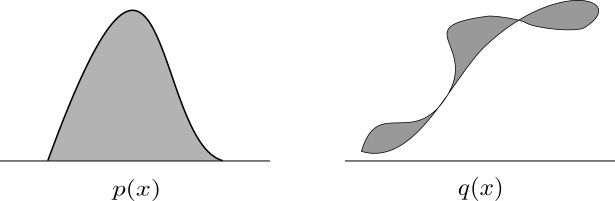
In order to get $ \small \text{KL} ( p \parallel q) = \mathbb{E}_{x \sim p(x)} \left[ \log \frac{p(x)}{q(x)} \right]$, we have to compute ratio $ \small \frac{p(x)}{q(x)}$ for all the points, but $ \small q(x)$ doesn’t even have density with respect to ambient space (thin line connects masses in figure 3.1). If we are interested in $ \small \text{KL} ( q \parallel p) = \mathbb{E}_{x \sim q(x)} \left[ \log \frac{q(x)}{p(x)} \right] $, when $ \small q(x) \rightarrow 0$ and $ \small p(x) > 0 $, the divergence shrinks to $ \small 0$, it means KL cannot measure the difference between distribution properly. In contrast, distances derived from optimal transport don’t have these problems.

OT and Wasserstein distance

Optimal transport is first introduced by Monge in 1781, Kantorovich later proposed a relaxation of the problem in early 20th century. We will revisit these mathematical formalism, then come up with Wasserstein distance, a special optimal transport cost that is widely used in recent generative models.

Monge’s Problem: Given measurable space $ \small \Omega$; a cost function $ \small c: \Omega \times \Omega \rightarrow \mathbb{R} $, $ \small \mu$ and $ \small \nu$ are 2 probability measures in $ \small \mathcal{P}(\Omega)$. Monge’s problem is to find a map $ \small T: \Omega \rightarrow \Omega$ such that:

\[\small \begin{align} \inf_{T_{\#}\mu = \nu} \int_{\Omega} c(x, T(x)) d\mu (x) \label{eq3.1} \tag{3.1} \end{align}\]

where $ \small T_{\#} \mu$ is push-forward operator, intuitively it moves entire distribution $ \small \mu$ to $ \small \nu$. Since $T$ does not always exist, Kantorovich consider probability couplings instead.

Kantorovich’s Problem (Primal): Given $ \small \mu$, $ \small \nu$ in $ \small \mathcal{P}(\Omega)$; a cost function $ \small c$ on $ \small \Omega \times \Omega$, the problem is to find a coupling $ \small \gamma \in \Gamma$ such that:

\[\small \begin{align} \inf_{\gamma \in \Gamma(\mu, \nu)} \iint_{\Omega \times \Omega} c(x, y) d\gamma(x, y) \label{eq3.2} \tag{3.2} \end{align}\]

where $ \small \Gamma$ is the set of probability couplings:

\[\small \begin{align*} \Gamma(\mu, \nu) \mathrel{\vcenter{:}}= \: & \{ \gamma \in \mathcal{P}(\Omega \times \Omega) \mid \forall A, B \subset \Omega, \\ &\gamma(A \times \Omega) = \mu(A), \\ &\gamma(B \times \Omega) = \nu(B) \} \end{align*}\]

Problem ($\ref{eq3.2}$) is primal form, it can be derived to duality formula. Given 2 real-valued functions $ \small \varphi$, $ \small \psi$ on $ \small \Omega$ such that:

\[\small \begin{align*} (\varphi \oplus \psi) (x, y) \mathrel{\vcenter{:}}= \varphi (x) + \psi(y) \end{align*}\]

then minimum of Kantorovich’s problem is equal to:

Kantorovich’s Problem (Duality):

\[\small \begin{align} \sup_{\varphi \oplus \psi \leq c } \int \varphi d \mu(x) + \int \psi d \nu (y) \label{eq3.3} \tag{3.3} \end{align}\]

Proof:
We have the followed function only takes 2 values:

\[\small g_{\Gamma}(\gamma) = \sup_{\varphi, \psi} \left[ \int \varphi d \mu + \int \psi d \nu - \iint \varphi \oplus \psi d \gamma \right] = \left\{ \begin{array}{lr} 0 \: & \text{if } \gamma \in \Gamma \\ +\infty \: & \text{otherwise} \end{array} \right.\]

Put it into ($\ref{eq3.2}$), the problem can be transformed to:

\[\small \begin{align*} \text{(\ref{eq3.2})} \Leftrightarrow & \inf_{\gamma \in \mathcal{P}_{+}(\Omega \times \Omega) } \iint c d \gamma + g_{\Gamma}(\gamma) \\ \Leftrightarrow & \inf_{\gamma \in \mathcal{P}_{+}(\Omega \times \Omega) } \left[ \iint c d \gamma + \sup_{\varphi, \psi} \left( \int \varphi d \mu + \int \psi d \nu - \iint \varphi \oplus \psi d \gamma \right) \right] \\ \Leftrightarrow & \inf_{\gamma \in \mathcal{P}_{+}(\Omega \times \Omega) } \sup_{\varphi, \psi} \left[ \iint \left( c - \varphi \oplus \psi \right) d \gamma + \int \varphi d \mu + \int \psi d \nu \right] \\ \Leftrightarrow & \sup_{\varphi, \psi} \inf_{\gamma \in \mathcal{P}_{+}(\Omega \times \Omega) } \left[ \iint \left( c - \varphi \oplus \psi \right) d \gamma + \int \varphi d \mu + \int \psi d \nu \right] \\ \Leftrightarrow & \sup_{\varphi, \psi} \left[ \inf_{\gamma \in \mathcal{P}_{+}(\Omega \times \Omega) } \iint \left( c - \varphi \oplus \psi \right) d \gamma + \int \varphi d \mu + \int \psi d \nu \right] \tag{$\star$} \end{align*}\]

But we know that:

\[\small \inf_{\gamma \in \mathcal{P}_{+}(\Omega \times \Omega) } \iint \left( c - \varphi \oplus \psi \right) d \gamma = \left\{ \begin{array}{lr} 0 \: & \text{if } c - \varphi \oplus \psi \geq 0 \\ -\infty \: & \text{otherwise} \end{array} \right.\]

Hence:

\(\small \begin{align*} (\star) \Leftrightarrow \sup_{\varphi \oplus \psi \leq c } \int \varphi d \mu + \int \psi d \nu \end{align*}\) ∎

When cost function $ \small c(x, y)$ is a metric $ \small D^p(x,y)$, optimal transport cost is simplified to $ \small p$-Wasserstein distance $ \small W_p$:

$p$-Wasserstein distance:

\[\small \begin{align} W_p (\mu, \nu) & \mathrel{\vcenter{:}}= \left( \inf_{\gamma \in \Gamma(\mu, \nu)} \iint D^p(x,y) d \gamma(x, y) \right)^{1/p} \label{eq3.4} \tag{3.4} \\ W_p^p (\mu, \nu) & \mathrel{\vcenter{:}}= \sup_{\varphi (x) + \psi (y) \leq D^p(x,y)} \int \varphi d \mu + \int \psi d \nu \label{eq3.5} \tag{3.5} \end{align}\]

Equations ($\ref{eq3.4}$) and ($\ref{eq3.5}$) are primal and duality forms respectively.

Assume $ \small \varphi$ is known, we would like to find a good $ \small \psi$ to solve ($\ref{eq3.5}$). Under this assumption, $ \small \psi$ must satisfy below condition:

\[\small \begin{align} \psi(y) \leq & \: D^p(x,y) - \varphi(x) \: \forall x, y \nonumber \\ \Leftrightarrow \psi(y) \leq & \: \inf_{x} D^p(x,y) - \varphi(x) =\mathrel{\vcenter{:}} \bar{\varphi}_x(y) \label{eq3.6} \tag{3.6} \end{align}\]

The R.H.S of ($\ref{eq3.6}$) is called $ \small D^p$-transform (of $ \small \varphi$); of course we might exchange $ \small \varphi$ for $ \small \psi$ and get the $ \small D^p$-transform of $ \small \psi$ instead. The duality of $ \small p$-Wasserstein now can be rewritten in semi-duality form:

\[\small \begin{align} W_p^p (\mu, \nu) = \sup_{\varphi} \int \varphi d \mu + \int \bar{\varphi} d \nu \label{eq3.7} \tag{3.7} \end{align}\]

Recall the definition of $ \small D^p$-concavity: a function $ \small \varphi (x)$ is $ \small D^p$-concave if there exists $ \small \phi(y)$ such that: $ \small \varphi(x) = \bar{\phi}(x)$ (where $ \small \varphi,\: \phi$ are “well-defined” on $ \small \Omega$).
Thus, if $ \small \varphi$ is $ \small D^p$-concave: $ \small \exists \phi \: \text{s.t. } \varphi(x) = \bar{\phi}(x) \implies \bar{\varphi}(y) = \phi(y) \implies \bar{\bar{\varphi}}(x) = \bar{\phi}(x) = \varphi(x) $. Put the constraint into ($\ref{eq3.7}$):

\[\small \begin{align} W_p^p (\mu, \nu) = \sup_{\varphi \: \text{is $D^p$-concave}} \int \varphi d \mu + \int \bar{\varphi} d \nu \label{eq3.8} \tag{3.8} \end{align}\]

In machine learning, we often take $ \small p=1$ and use $\small 1$-Wasserstein distance to measure the discrepancy between distributions, the duality form becomes:

\[\small \begin{align} W_1 (\mu, \nu) = \sup_{\varphi \: \text{is $1$-Lipschitz}} \int_{\Omega} \varphi (d\mu - d\nu) \label{eq3.9} \tag{3.9} \end{align}\]

To arrive ($\ref{eq3.9}$), we must show that: $ \small p=1$ and $ \small \varphi$ is concave $ \small \Leftrightarrow$ $\bar{\varphi} = - \varphi$ and $ \small \varphi$ is $ \small 1$-Lipshitz

Proof:
Define $ \small \bar{\varphi}_x(y) \mathrel{\vcenter{:}}= D(x,y) - \varphi(x)$, obviously:
\(\small \bar{\varphi}_x(y) - \bar{\varphi}_x(y^{\prime}) = D(x,y) - D(x,y^{\prime}) \leq D(y,y^{\prime}) \implies \varphi_x(y) \: \text{is 1-Lipschitz}\)
\(\small \implies \bar{\varphi}(y) = \inf_{x}\bar{\varphi}_x(y) \: \text{is 1-Lipschitz}\)
\(\small \implies \bar{\varphi}(y) - \bar{\varphi}(x) \leq D(x,y)$ $\implies -\bar{\varphi}(x) \leq D(x,y) - \bar{\varphi}(y)\)
\(\small \implies -\bar{\varphi}(x) \leq \inf_{y} D(x,y) - \bar{\varphi}(y)\)
\(\small \implies -\bar{\varphi}(x) \leq \inf_{y} D(x,y) - \bar{\varphi}(y) \leq -\bar{\varphi}(x)\)
\(\small \implies -\bar{\varphi}(x) \leq \bar{\bar{\varphi}}(x) \leq -\bar{\varphi}(x) \implies \bar{\varphi}(x) = -\bar{\bar{\varphi}}(x) = -\varphi(x)\) ∎

One interested in detailed proofs can refer to (Gabriel Peyre and Marco Cuturi, 2018) and Cuturi’s talk.
Side note: Discriminator of Wasserstein GAN serves as function $\varphi$ of semi-duality form (Genevay et al,, 2017), $ \small 1$-Lipschitz constraint is fulfilled by weight-clipping (WGAN, Arjovsky et al., 2017) or gradient-penalizing (WGAN-GP, Gulrajani et al., 2017).

Empirical Wasserstein distance

We have briefly covered basics of optimal transport. Solving OT is rather problematic except for certain cases, e.g. univariate or Gaussian measures. Our primary objective is to efficiently compute Wasserstein distance on empirical measures which appear in probabilistic models frequently.

We consider 2 measures $ \small \mu=\sum_{i=1}^{n} a_{i} \delta_{x_{i}}$ and $ \small \nu=\sum_{j=1}^{m} b_{j} \delta_{y_{j}}$ where $\delta_{x_{i}}$, $ \small \delta_{y_{j}}$ are Dirac functions at $ \small x_i$, $ \small y_j$ respectively. In this particular case, cost function and coupling set are specified as:

\[\small \begin{align} M_{X Y} \mathrel{\vcenter{:}}=& \left[D\left(x_{i}, y_{j}\right)^{p}\right]_{i j} \nonumber \\ U(a, b) \mathrel{\vcenter{:}}=& \left\{P \in \mathbb{R}_{+}^{n \times m} | P \mathbf{1}_{m}=a, P^{T} \mathbf{1}_{n}=b\right\} \nonumber \end{align}\]

We then can substitute Frobenius inner product for integral in OT’s primal form:

\[\small \begin{align} & W_{p}^{p}(\mu, \nu)=\min _{P \in U(a, b)}\left\langle P, M_{X Y}\right\rangle \label{eq3.10} \tag{3.10} \\ \text{where:} \: & \left\langle \cdot, \cdot \right\rangle \: \text{is } \href{https://en.wikipedia.org/wiki/Frobenius_inner_product}{\text{Frobenius inner product}} \nonumber \end{align}\]

Dual form:

\[\small \begin{align} W_{p}^{p}(\mu, \nu)=\max _{\alpha \in \mathbb{R}^{n}, \beta \in \mathbb{R}^{m}} \alpha^{T} a+\beta^{T} b \label{eq3.11} \tag{3.11} \end{align}\]

One challenge is that solution of ($\ref{eq3.10}$), ($\ref{eq3.11}$) is unstable and not always unique (Cuturi’s, 2019). Additionally, $ \small W_p^p$ is not differentiable, making training models by stochastic gradient optimization less feasible. Fortunately, entropic regularization which is used to measure the level of uncertainty in a probability distribution can overcome these disadvantages:

Entropic Regularization: For joint distribution $ \small P(x, y)$ (in this section, we only concern about discrete distribution unless stated otherwise):

\[\small \begin{align*} \mathcal{H}(P) \mathrel{\vcenter{:}}= - \sum_{i} \sum_{j} P(x_i,y_j) \log P(x_i,y_j) \end{align*}\]

For particular $\small P \in U(a,b)$ :

\[\small \mathcal{H}(P) = -\sum_{i,j=1}^{n,m} P(x_i,y_j) \left(\log P(x_i,y_j) -1 \right) = \sum_{i,j=1}^{n,m} P_{ij} \left(\log P_{ij} -1 \right)\]

Regularized Wasserstein:

\[\small \begin{align} & W_{\epsilon}(\mu, \nu) = \min _{P \in U(a, b)} \left\langle P, M_{X Y}\right\rangle - \epsilon \mathcal{H}(P) \label{eq3.12} \tag{3.12} \\ \text{where:} \: & \epsilon \geq 0 \: \text{is regularization coeficient} \nonumber \end{align}\]

Strong concavity property of entropic regularization ensures the solution of ($\ref{eq3.12}$) is unique. Moreover, it can lead to a differentiable solution using Sinkhorn’s algorithm. To come up with Sinkhorn iteration, we need an additional proposition.

Prop.1: If $ \small P_{\epsilon} \mathrel{\vcenter{:}}= \arg \min_{P \in U(a, b)} \left\langle P, M_{X Y}\right\rangle - \epsilon \mathcal{H}(P) $ then: $ \small \exists ! u \in \mathbb{R}_{+}^{n}, v \in \mathbb{R}_{+}^{m} $ such that:

\[\small \begin{align*} P_{\epsilon}=\operatorname{diag}(u) K \operatorname{diag}(v) \: \text{with} \: K \mathrel{\vcenter{:}}= e^{-M_{X Y} / \epsilon} \end{align*}\]

Proof:
We have:

\[\small L(P, \alpha, \beta) = \sum_{i j} P_{i j} M_{i j} + \epsilon P_{i j}\left(\log P_{i j}-1\right)+\alpha^{T}(P \mathbf{1}-a)+\beta^{T}\left(P^{T} \mathbf{1}-b\right)\] \[\small \frac{\partial L}{\partial P_{ij}} = M_{i j} + \epsilon \log P_{ij} + \alpha_i + \beta_j\]

Set this partial derivative equal to $ \small 0$, we get:

\[\small P_{i j}=e^{\frac{\alpha_{i}}{\epsilon}} e^{-\frac{M_{i j}}{\epsilon}} e^{\frac{\beta_{j}}{\epsilon}}=u_{i} K_{i j} v_{j}\]

hence:

\[\small P_{\epsilon} \in U(a, b) \Leftrightarrow \left\{ \begin{array}{ll} {\operatorname{diag}(u) K \operatorname{diag}(v) \mathbf{1}_{m}} & {=a} \\ {\operatorname{diag}(v) K^{T} \operatorname{diag}(u) \mathbf{1}_{n}} & {=b} \end{array} \right.\] \[\small \implies P_{\epsilon} \in U(a, b) \Leftrightarrow \left\{ \begin{array}{ll} {\operatorname{diag}(u) K v} & {=a} \\ {\operatorname{diag}(v) K^{T} u } & {=b} \end{array} \right.\] \[\small \implies P_{\epsilon} \in U(a, b) \Leftrightarrow \left\{ \begin{array}{ll} {u \odot K v} & {=a} \\ {v \odot K^{T} u } & {=b} \end{array} \right.\]

\(\small \implies \left\{ \begin{array}{ll} {u} & {= a / Kv} \\ {v} & {= b / K^Tu} \end{array} \right.\) ∎

The above prop. suggests that if there exists a solution for regularized Wasserstein, it is unique and possibly computed once $ \small u, v$ are available. As seen in the proof, these quantities can be approximated by repeating the last equation. In detail:

Sinkhorn’s algorithm: Input $ \small M_{XY}, \: \epsilon, \: a, \: b$. Initialize $ \small u, \: v$. Calculate $ \small K = e^{-M_{XY}/\epsilon}$. Repeat until convergence:

\[\small \begin{align} \begin{array}{ll} u &= a / Kv \\ v &= b / K^Tu \end{array} \label{eq3.13} \tag{3.13} \end{align}\]

Clearly, Sinkhorn iteration is differentiable.

Sinkhorn’s algorithm involves with a number of other measures in OT but we will skip them since it is irrelevant to the next section, Wasserstein distance in VI. One last thing to remember is that when regularization coefficient $ \small \epsilon$ tends to infinity, Sinkhorn’s distance turns into Maximum Mean Discrepancy (MMD) distance.

Part 4