Optimal Transport and Variational Inference (part 4)

Part 3

VI with Wasserstein distance

We now have enough materials to study VI models whose objective functions are derived from Wasserstein distance. The first three models we look at are Wasserstein Autoencoders (WAE) and its variants, Sinkhorn Autoencoders (SAE) and Sliced-WAE. The last one we consider is Wasserstein Variational Inference (WVI) whose cost function is different from the other three.

Wasserstein Autoencoders

WAE (Tolstikhin et al., 2018) is similar to VAE in both model-architecture and target-function. In structural term, WAE and VAE both employ 2 neural networks, one is encoder that encodes data into latent variables, another is decoder that reconstructs data from learned latent representation. In term of target, they both aim to minimize the reconstruction loss and regularize latent variables. The difference is that WAE takes Wasserstein distance instead of KL divergence as its objective (recall that VAE tries to maximize a marginal log-likelihood which leads to KL loss).

Given observation $ \small X \in \mathcal{X}$ with distribution $ \small P_X$, WAE models data by introducing latent variable $ \small Z \in \mathcal{Z}$ with prior $ \small P_Z$. The inference network $ \small Q_Z(Z|X)$, i.e. encoder, learns $ \small Z$ from $ \small X$ whilst generative network $ \small P_G(X|Z)$,i.e. decoder, reconstructs data from latent variables. Marginal distribution $ \small Q_Z$ of $ \small Z$ can be obtained through inference model when $ \small X \sim P_X$ and $ \small Z \sim Q_Z(Z|X)$. It can be expressed in a form of density:

\[\small \begin{align*} q_Z(z) = \int_{\mathcal{X}} q_Z(z|x) p_X(x) dx \end{align*}\]

Similarly, latent variable model $ \small P_G$ can be defined by $ \small Z \sim P_Z$ and conditional distribution $ \small P_G(X|Z)$:

\[\small \begin{align*} p_G(x) = \int_{\mathcal{Z}} p_G(x|z) p_Z(z) dz \end{align*}\]

WAE focuses on deterministic $ \small P_G(X|Z)$, i.e. decoder deterministically maps $ \small Z$ to $ \small X$ by a function $ \small G(Z)$:

\[\small \begin{align*} G: & \mathcal{Z} \rightarrow \mathcal{X} \\ & Z \mapsto X \end{align*}\]

The goal of WAE is to minimize Wasserstein distance between $ \small P_X$ and $ \small P_G(X)$ distributions. Additionally, we will see later that this distance also measures the discrepancy between $ \small Q_Z(Z)$ and $ \small P_Z$. In other words, it conveniently contains both reconstruction cost and regularization term. WAE’s objective bases on the next theorem.

Theorem 4.1: For deterministic $ \small P_G(X|Z)$, $ \small Q_Z$, $ \small P_G$ and any function $ \small G$ defined above, we have:

\[\small \begin{align*} \inf _{\Gamma \in \mathcal{P}\left(X \sim P_{X}, Y \sim P_{G}\right)} \mathbb{E}_{(X, Y) \sim \Gamma}[c(X, Y)]=\inf _{Q : Q_{Z}=P_{Z}} \mathbb{E}_{P_{X}} \mathbb{E}_{Q(Z | X)}[c(X, G(Z))] \end{align*}\]

The L.H.S is exactly the primal form of Wasserstein distance between $ \small P_G$ and $ \small P_X$. By Lagrange multiplier, we can rewrite the problem to arrive with WAE’s objective:

\[\small \begin{align} & \mathcal{L}_{\mathrm{WAE}}\left(P_{X}, P_{G}\right) :=\inf _{Q(Z | X) \in \mathcal{Q}} \mathbb{E}_{P_{X}} \mathbb{E}_{Q(Z | X)}[c(X, G(Z))]+\lambda \cdot \mathcal{D}_{Z}\left(Q_{Z}, P_{Z}\right) \label{eq4.1} \tag{4.1} \\ \text{where:} & \: \mathcal{Q} \: \text{is any nonparametric set of probabilistic encoders} \nonumber \\ & \: \lambda > 0 \: \text{is a hyperparameter} \nonumber \\ & \: \mathcal{D}_{Z} \: \text{is any divergence} \nonumber \end{align}\]

In the paper, $ \small c$ is set as $ \small L_2-norm$. Because gradients of latent variables (w.r.t model’s parameters) are necessary for stochastic gradient optimization, $ \small \mathcal{D}_Z$ should be non-difficult to compute/estimate these gradients. The authors consider 2 options. The first choice of $ \small \mathcal{D}_Z$ is Jensen-Shannon divergence $ \small \mathcal{D}_{JS}$; the second is MMD.

In former case, $ \small \mathcal{D}_{JS}$ is estimated by adversarial training on latent samples. It turns into min-max problem, similar to GAN, but on latent space instead:

    
\begin{algorithm}
\caption{GAN-based}
\begin{algorithmic}
\REQUIRE Regularization coefficient $\lambda > 0$, \\
	Encoder $Q_\phi$, decoder $G_\theta$, latent discriminator $D_\gamma$
\WHILE{($\phi$, $\theta$) not converged}
	\STATE Sample $\{ x_1, \dots, x_n \}$ from training set
	\STATE Sample $\{ z_1, \dots, z_n \}$ from $P_Z$
	\STATE Sample $\tilde{z}_i$ from $Q_\phi (Z|x_i)$ for $i=1,\dots,n$
	\STATE Update $D_\gamma$ by ascending:
	\STATE $\qquad \frac{\lambda}{n} \sum_{i=1}^{n} \log D_{\gamma}\left(z_{i}\right)+\log\left(1-D_{\gamma}\left(\tilde{z}_{i}\right)\right)$
	\STATE Update $Q_\phi, \: G_\theta$ by descending:
	\STATE $\qquad \frac{1}{n} \sum_{i=1}^{n} c\left(x_{i}, G_{\theta}\left(\tilde{z}_{i}\right)\right)-\lambda \cdot \log D_{\gamma}\left(\tilde{z}_{i}\right)$
\ENDWHILE
\end{algorithmic}
\end{algorithm}

In later case, a characteristic positive-definite kernel $ \small k: \mathcal{Z} \times \mathcal{Z} \rightarrow \mathcal{X}$ is used to define MMD:

\[\small \begin{align*} & \operatorname{MMD}_{k}\left(P_{Z}, Q_{Z}\right)=\left\|\int_{\mathcal{Z}} k(z, \cdot) d P_{Z}(z)-\int_{\mathcal{Z}} k(z, \cdot) d Q_{Z}(z)\right\|_{\mathcal{H}_{k}} \\ \text{where:} & \: {\mathcal{H}_{k}} \: \text{is the RKHS} \end{align*}\]

Since MMD has an unbiased U-statistic estimator, it allows estimating gradient. Training procedure of MMD-based:

    
\begin{algorithm}
\caption{MMD-based}
\begin{algorithmic}
\REQUIRE Regularization coefficient $\lambda > 0$, \\
	Encoder $Q_\phi$, decoder $G_\theta$, \\
	characteristic positive-definite kernel $k$
\WHILE{($\phi$, $\theta$) not converged}
	\STATE Sample $\{ x_1, \dots, x_n \}$ from training set
	\STATE Sample $\{ z_1, \dots, z_n \}$ from $P_Z$
	\STATE Sample $\tilde{z}_i$ from $Q_\phi (Z|x_i)$ for $i=1,\dots,n$
	\STATE Update $Q_\phi, \: G_\theta$ by descending:
	\STATE $\qquad \frac{\lambda}{n} \sum_{i=1}^{n} \log D_{\gamma}\left(z_{i}\right)+\log\left(1-D_{\gamma}\left(\tilde{z}_{i}\right)\right)$
	\STATE Update $Q_\phi, \: G_\theta$ by descending:
	\STATE $\qquad \frac{1}{n} \sum_{i=1}^{n} c\left(x_{i}, G_{\theta}\left(\tilde{z}_{i}\right)\right)+\frac{\lambda}{n(n-1)} \sum_{\ell \neq j} k\left(z_{\ell}, z_{j}\right) +\frac{\lambda}{n(n-1)} \sum_{\ell \neq j} k\left(\tilde{z}_{\ell}, \tilde{z}_{j}\right)-\frac{2 \lambda}{n^{2}} \sum_{\ell, j} k\left(z_{\ell}, \tilde{z}_{j}\right)$
\ENDWHILE
\end{algorithmic}
\end{algorithm}

While decoder of VAE could not be deterministic (otherwise it falls back to ordinary auto-encoder), $ \small Q_\phi(Z|X)$ in algorithms 4.1, 4.2 can be non-random, i.e. WAE’s decoder can deterministically map each $ \small x_i$ to $ \small \tilde{z}_i$.

Sinkhorn AE

Sinkhorn AE (Patrini et al., 2019) has the same objective as WAE except the regularization on latent space. In stead of GAN-based or MMD-based, SAE minimizes a Wasserstein distance between $ \small Q_Z$ and $ \small P_Z$, i.e. $ \small \mathcal{D}_Z$ is Wasserstein distance. But computing Wasserstein on continuous distribution is very challenging, SAE overcomes this problem by considering samples from such distribution as Dirac deltas, i.e. estimating empirical distributrion from its samples. Since expectation of Dirac function defines a discrete distribution, it allows us to approximate Wasserstein distance by differentiable Sinkhorn iteration (section optimal transport).

Given 2 discrete distributions on support of $ \small M$ points $ \small \hat{P} = \frac{1}{M} \sum_{i=1}^{M} \delta_{z_{i}}$, $\hat{Q}= \frac{1}{M} \sum_{i=1}^{M} \delta_{\tilde{z}_{i}}$. Follow 3.10, empirical Wasserstein distance associated with cost function $ \small c’$ is:

\[\small \begin{align} & W_{c'} (\hat{Q}, \hat{P}) = \frac{1}{M} \min_{R \in S_M} \left\langle R, C' \right\rangle \label{eq4.2} \tag{4.2} \\ \text{where: } & C'_{ij} = c'(\tilde{z}_i, z_j) \nonumber \\ & S_M = \{ R \in \mathbb{R}_{\geq 0}^{M \times M} \mid R\mathbf{1} = \mathbf{1}, R^T\mathbf{1} = \mathbf{1} \} \nonumber \end{align}\]

Adding entropic regularization $ \small \mathcal{H}(R) = - \sum_{i,j=1}^{M,M} R_{i,j} \log R_{i, j} $ to this distance, we arrive with Sinkhorn distance:

\[\small \begin{align} & S_{c', \epsilon} (\hat{Q}, \hat{P}) = \min_{R \in S_M} \left\langle R, C' \right\rangle - \epsilon \mathcal{H}(R) \label{eq4.3} \tag{4.3} \\ \text{where: } & \epsilon > 0 \text{ is coefficient} \nonumber \end{align}\]

From theoretical perspective, SAE works thanks to below theorems.

Theorem 4.2: If $ \small G(Z|X)$ is deterministic and $ \small \gamma-Lipschitz$ then:

\[\small \begin{align*} W_p(P_X, P_G) \leq W_p(P_X, G_{\#} Q_Z) + \gamma W_p(Q_Z, P_Z) \end{align*}\]

If $ \small G(Z|X) $ is stochastic, the result holds with $ \small \gamma = \sup_{\mathcal{P} \neq \mathcal{Q}} \frac{ W_p (G(X|Z)_{\#} \mathcal{P}, W_p (G(X|Z)_{\#} \mathcal{Q})} {W_p(\mathcal{P}, \mathcal{Q})}$

Theorem 4.3: Let $ \small P_X$ is not anatomic and $ \small G(X|Z)$ is deterministic. Then for every continuous cost $ \small c$:

\[\small \begin{align*} W_c(P_X, P_G) = \inf_{Q(Z | X) \text{ dertministic: } Q_Z=P_Z} \mathbb{E}{X \sim P_X} \mathbb{E}{Z \sim Q(Z|X)} c(X, G(Z)) \end{align*}\]

Using the cost $ \small c(x,y) = {\lVert}{x - y}{\rVert}_2^p $, the equation holds with $ \small W_p^p(P_X,P_G)$ in place of $W_c(P_X,P_G)$

Theorem 4.4: Suppose perfect reconstruction, that is, $ \small P_X = (G \circ Q)_{\#}P_X $. Then:

\[\small \begin{align*} \text{i)} \: P_Z = Q_Z \implies P_X = P_G \\ \text{ii)} \: P_Z \neq Q_Z \implies P_X \neq P_G \end{align*}\]

By theorem 4.2, Wasserstein distance between data and generative model distributions has an upper bound, minimizing this bound leads to minimizing discrepancy between $ \small P_X$ and $ \small P_G$. Furthermore, the upper bound includes Wasserstein distance between aggregated posterior and the prior, we can estimate this distance by Sinkhorn on their samples. Theorem 4.3 allows us to have an deterministic auto-encoders, i.e. both $ \small G(X|Z)$ and $ \small Q(Z|X)$ are deterministic. The last one, theorem 4.4 means that under perfect-reconstruction assumption, matching aggregated posterior and prior is: (i) sufficient and (ii) necessary to model data distribution. This theorem reminds us to choose proper prior. Previous research have shown that the choice of prior should encourage geometric properties of latent space since it provides remarkable performance of representation learning. The authors consider few options: spherical, Dirichlet prior.

Finally, Sinkhorn algorithm for estimating Wasserstein distance between $ \small Q_Z$ and $ \small P_Z$:

    
\begin{algorithm}
\caption{Sharp Sinkhorn}
\begin{algorithmic}
\REQUIRE $\{z_i \}_{i=1}^m, \: \{ \tilde{z}_i \}_{i=1}^m , \: \epsilon > 0, \: L > 0 \: \forall i,j $ \\
	$C_{ij} = c(z_i, \tilde{z}_j), \: K=e^{-C/\epsilon}, \: u \leftarrow \mathbf{1}$
\FOR{$L$ times}
	\STATE $\qquad v \leftarrow \mathbf{1}/(K^Tu) \quad$ \#element-wise division
	\STATE $\qquad u \leftarrow \mathbf{1}/(Kv) $
\ENDFOR
\STATE $R \leftarrow \operatorname{Diag}(u) K \operatorname{Diag}(v) $
\RETURN $\frac{1}{M} \langle C,R \rangle $
\end{algorithmic}
\end{algorithm}

Sliced-WAE

Sliced-WAE (Kolouri et al., 2018) yields another way to minimize the discrepancy between aggregated posterior $\small Q_Z$ and prior distributions $\small P_Z$. Similar to SAE, Sliced-WAE measures this discrepancy by Wasserstein distance but utilizes different approximation algorithm. It is based on the fact that computing this distance of univariate distributions is analytically simple. Hence, Sliced-WAE approximates Wasserstein distance on high-dimensional space through 2 steps: (1) projecting its distributions into sets of one-dimensional distributions, (2) estimating the original distance via Wasserstein distances of projected representations.

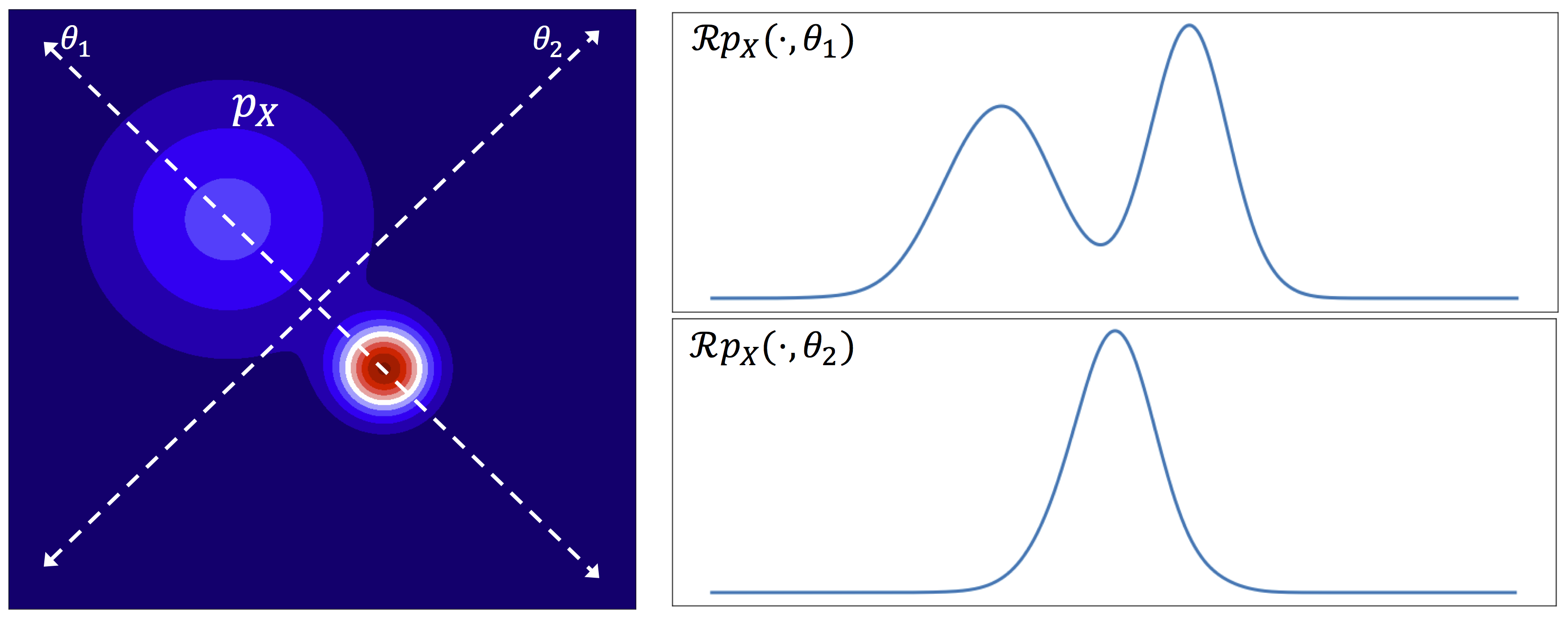
To project high-dimensional distribution on one-dimensional space, it uses Radon transform:

\[\small \begin{align} &\mathcal{R}p_X(t;\theta) = \int_{\mathcal{X}} p_X(x) \delta(t - x \cdot \theta) dx, \quad \forall \theta \in \mathbb{S}^{d-1, \: \forall t \in \mathbb{R} } \label{eq4.4} \tag{4.4} \\ \text{where: } & \mathbb{S}^{d-1} \text{ is } d\text{-dimensional unit sphere} \nonumber \end{align}\]

For a fixed $ \small \theta \in \mathbb{S}^{d-1}$, $\small \mathcal{R}p_X(\cdot; \theta) = \int_{\mathbb{R}} \mathcal{R}p_X(t; \theta)dt $ is an one-dimensional slice of distribution $ \small p_X$, it can be obtained by integrating $ \small p_X$ over hyperplane orthogonal to $ \small \theta$. Fig 4.1 visualizes the projection with different $ \small \theta$s:

_{Fig4.1: Distribution slicing. (Source: Kolouri et al., 2018. ).}

A tricky situation is that only samples of distribution are observed. In such case, we can estimate and transform their empirical distributions (just like Sinkhorn VAE). Suppose $ \small x_m \sim p_X, \: m=1,\dots,M$, empirical distribution and its projection are:

\[\small \begin{align} &p_{X}^{*} = \frac{1}{M} \sum_{m=1}^{M} \delta_{x_m} \nonumber \\ &\mathcal{R} p_{X}^{*}(t, \theta)=\frac{1}{M} \sum_{m=1}^{M} \delta\left(t-x_{m} \cdot \theta\right), \: \forall \theta \in \mathrm{S}^{d-1}, \: \forall t \in \mathbb{R} \label{eq4.4a} \tag{4.4a} \end{align}\]

Recall the Wasserstein of univariate distributions: let $ \small F_X$, $ \small F_Y$ correspondingly be cumulative distribution function of densities $ \small p_X$, $ \small p_Y$ on sample space $ \small \mathbb{R}$, transport cost $ \small c(x,y)$ is convex. The closed-form of Wasserstein distance between these 2 distributions is:

\[\small \begin{align} W_c(p_X, p_Y) = \int_{0}^{1} c(F_X^{-1}(t), F_Y^{-1}(t)) dt \label{eq4.5} \tag{4.5} \end{align}\]

As equation ($\ref{eq4.5}$), the Wasserstein distance between $ \small p_X$ and $ \small p_Y$ can be expressed as:

\[\small \begin{align} SW_c(p_X, p_Y) = \int_{\mathbb{S}^{d-1}} c( \mathcal{R}p_X(\cdot; \theta), \mathcal{R}p_Y(\cdot; \theta) ) d\theta \label{eq4.6} \tag{4.6} \end{align}\]

When $ \small c = {\lVert}{x-y}{\rVert}_2^2$, we are allowed to approximate $ \small W_2$ by $ \small SW_2$ due to following inequalities:

\[\small \begin{align} & SW_2 (p_X, p_Y) \leq W_2 (p_X, p_Y) \leq \alpha SW_2^\beta (p_X, p_Y) \nonumber \\ \text{where: } & \alpha \text{ is a constant} \nonumber \\ & \beta = (2(d+1))^{-1} \: \text{ (refer } \href{https://arxiv.org/abs/1705.07642}{Bousquet \textit{et al.}} \text{ for proof)} \nonumber \end{align}\]

Thus if every sliced Wasserstein distance is calculated, then by ($\ref{eq4.6}$), Wasserstein distance of non-projected distributions can be accomplished.

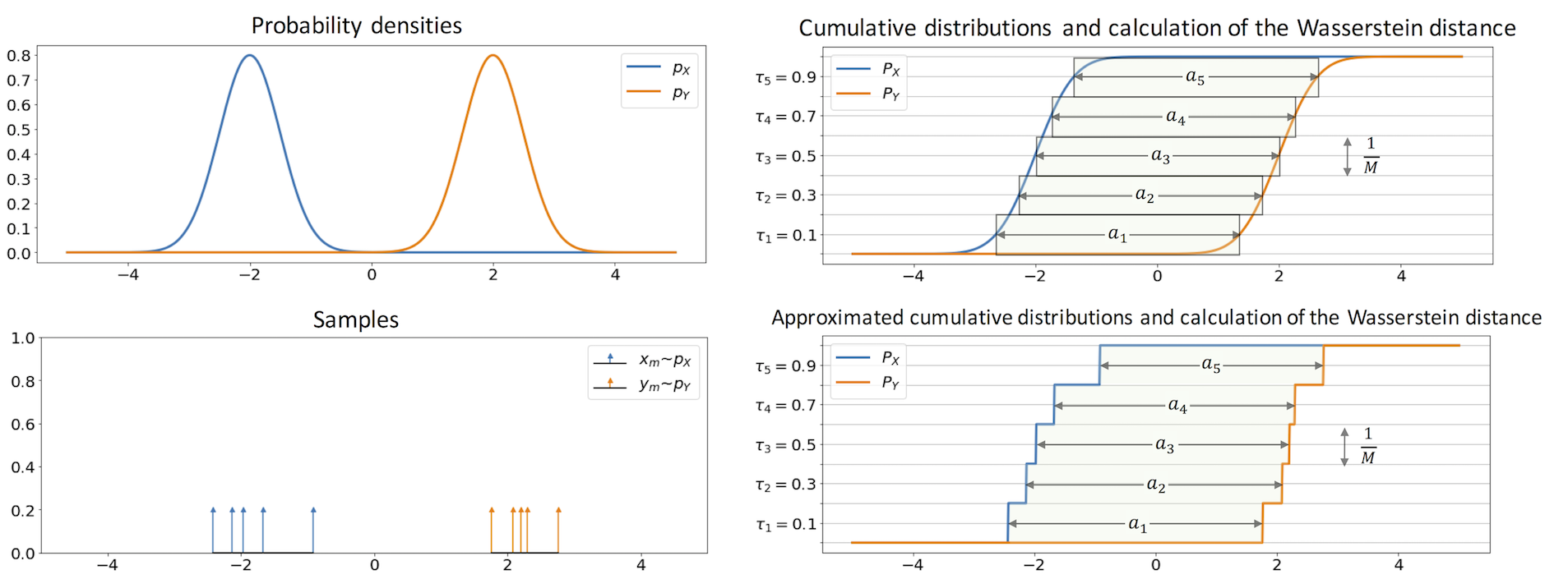
Assume $ \small p_X$, $ \small p_Y$ are 2 one-dimensional densities and we only have their samples $ \small x_m \sim p_X$, $ \small y_m \sim p_Y$. Same as Sinkhorn AE, $ \small p_{X}^{*} = \frac{1}{M} \sum_{m=1}^{M} \delta_{x_m}$ and $p_{Y}^{*} = \frac{1}{M} \sum_{m=1}^{M} \delta_{y_m}$ are empirical distributions. It results their cumulative distribution functions as $ \small P_X(t) = \frac{1}{M} \sum_{m=1}^{M} u(t-x_m) $, $ \small P_Y(t) = \frac{1}{M} \sum_{i=1}^{M} u(t-y_m) $ where $ \small u(\cdot)$ is step function. If we sort $ \small x_m$s in ascending order, i.e. $ \small x_{i[m]} \leq x_{i[m+1]}$ where $ \small i[m]$ is index of sorted $ \small x_m$s, clearly we achieve $ \small P_X^{-1} (\tau_m) = x_{i[m]} $. Hence, for sorted $ \small x_m$s and $ \small y_m$s, the Wasserstein distance is:

\[\small \begin{align} W_c(p_X, p_Y) \approx \frac{1}{M} \sum_{m=1}^{M} c(x_{i[m]}, y_{j[m]} ) \label{eq4.7} \tag{4.7} \end{align}\]

On the other hand, if $ \small p_X$ and $ \small p_Y$ are already known, ($\ref{eq4.6}$) can be numerically calculated without their samples by using $ \small \frac{1}{M} \sum_{m=1}^{M} a_m $ with $ \small a_m = c(P_X^{-1}(\tau_m), P_Y^{-1}(\tau_m))$, $ \small \tau_m = \frac{2m-1}{2M}$ (see the figure 4.2).

_{Fig4.2: Top row: one-dimensional distribution densities are known (top left), the Wasserstein distance then can be analytically computed (top right). Bottom row: only samples of distributions are available (bottom left), then $a_m = c(x_{i[m]}. y_{j[m]})$ where $x_{i[m]}. y_{j[m]}$ are sorted in ascending order (bottom right). (Source: Kolouri et al., 2018. ).}

Combine ($\ref{eq4.4a}$), ($\ref{eq4.6}$) and ($\ref{eq4.7}$) together, the discrepancy between $ \small P_Z$ and $ \small Q_Z$ can be measured by sliced Wasserstein distance $ \small SW_c(P_Z, Q_Z)$. But the integration over $ \small d$-dimensional unit sphere $ \small \mathbb{S}^{d-1}$ (often $ \small \mathbb{R}^d$) in ($\ref{eq4.6}$) is practically expensive. The solution is to substitute it with following summation:

\[\small \begin{align} SW_c(Q_Z, P_Z) \approx \frac{1}{{\lvert}{\Theta}{\rvert}} \sum_{\theta_l \in \Theta} W_c(\mathcal{R}q_Z(\cdot;\theta_l), \mathcal{R}p_Z(\cdot;\theta_l)) \label{eq4.8} \tag{4.8} \\ \text{where: } \Theta \text{ is finite set and } \Theta \subset \mathbb{S}^{d-1} \nonumber \end{align}\]

Finally, Sliced-WAE algorithm for training procedure:

    
\begin{algorithm}
\caption{Sliced-WAE}
\begin{algorithmic}
\REQUIRE Regularization coefficient $\lambda$, \\
	number of random projections $L$ \\
	Encoder $\phi$, decoder $\psi$
\WHILE{$\phi$, $\psi$ not converged}
	\STATE Sample $\{x_1, \dots, x_M \}$ from training set
	\STATE Sample $\{z_1, \dots, z_M \}$ from prior $P_Z$
	\STATE Sample $\{\theta_1, \dots, \theta_L \}$ from $\mathbb{S}^{K-1}$
	\STATE Sort $\theta_l \cdot z_m$ s.t. $\theta_l \cdot z_{i[m]} \leq \theta_l \cdot z_{i[m+1]}$
	\STATE Sort $\theta_l \cdot \phi(x_m)$ s.t. $\theta_l \cdot \phi(x_{j[m]}) \leq \theta_l \cdot \phi(x_{j[m+1]})$
	\STATE Update $\phi$ and $\psi$ by descending:
	\STATE $\qquad \sum_{m=1}^{M}c(x_m, \psi(\phi(x_m))) + \lambda \sum_{l=1}^{L} \sum_{m=1}^{M} c(\theta_l \cdot z_{i[m]}, \theta_l \cdot \phi(x_{j[m+1]}))$
\ENDWHILE
\end{algorithmic}
\end{algorithm}

Wasserstein VI (WVI)

Although WVI (Ambrogioni et at., 2018) also utilizes Wasserstein distance, its objective is different from above approaches. In particular, WVI adapts joint-contrastive variational inference by considering a divergence between joint distributions, i.e. $ \small \mathcal{D}(p(x,z) \parallel q(x,z))$ (while classic VI is referred as posterior-contrastive). Using Wasserstein distance as the divergence, WVI’s objective is to minimize the following loss:

\[\small \begin{align} &\mathcal{L}_{WVI} (p,q) = W_c(p(x,z), q(x,z)) = \inf_{\gamma \in \Gamma(p,q)} \int c(x, z; \tilde{x},\tilde{z}) d\gamma(x, z; \tilde{x},\tilde{z}) \label{eq4.9} \tag{4.9} \\ \text{where: }& x, z \sim p(x,z) \text{ and } \tilde{x},\tilde{z} \sim q(x,z) \nonumber \\ &\Gamma \text{ is set of probability couplings.} \nonumber \end{align}\]

In practice, when only samples are available, it fall-backs to computing the Wasserstein distance of 2 empirical distributions:

\[\small \begin{align} &\mathcal{L}_{WVI} (p_n,q_n) = \inf_{\gamma \in \Gamma(p,q)} \sum_{j,k} c(x_j, z_j;\tilde{x}_k, \tilde{z}_k) \gamma (x_j, z_j;\tilde{x}_k, \tilde{z}_k) \label{eq4.10} \tag{4.10} \\ \text{where: }& x_j, z_j \sim p(x,z) \text{ and } \tilde{x}_k, \tilde{z}_k \sim q(x,z) \nonumber \\ &p_n,q_n \text{ are empirical distributions estimated from } n \text{ samples} \nonumber \end{align}\]

The Wasserstein distance of joint-distributions can be estimated by its empirical Wasserstein distance (thus Monte Carlo estimator of its gradient can be obtained) thanks to following theorem:
Theorem 4.5: Let $ \small W_c(p_n, q_n)$ is the Wasserstein distance between two empirical distributions $ \small p_n, q_n$. For $n$ tends to infinity, there exists a positive number $s$ such that:

\[\small \begin{align*} \mathbb{E}{pq}\left[ W_c(p_n, q_n) \right] \lesssim W_c(p,q) + n^{-1/s} \end{align*}\]

See (Ambrogioni et at., 2018) for its proof.
Since Monte Carlo method is biased with finite value of $n$, to obtain an unbiased gradient estimator, we need to modify the objective to eliminate bias:

\[\small \begin{align} \tilde{\mathcal{L}}_c(p_n, q_n) = \mathcal{L}_c(p_n, q_n) - \frac{1}{2} \left( \mathcal{L}_c(p_n, p_n) + \mathcal{L}_c(q_n, q_n) \right) \label{eq4.11} \tag{4.11} \end{align}\]

It is clear that $ \small \mathbb{E}_{pq}[\tilde{\mathcal{L}}_c(p_n, q_n)] = 0 $ if $ \small p=q$ and furthermore, $ \small \lim_{n \rightarrow \infty}\tilde{\mathcal{L}}_c(p_n, q_n) = \mathcal{L}(p,q) $.

As we have seen in previous sections, $ \small \tilde{\mathcal{L}}_c(p_n, q_n)$ can be approximated by Sinkhorn algorithm 4.3. Since Sinkhorn iteration is differentiable, we have:

\[\small \begin{align} & \nabla \tilde{\mathcal{L}}_c(p_n, q_n) = \nabla S_{c,\epsilon}^t(p_n, q_n) \label{eq4.12} \tag{4.12} \\ \text{where: }& \epsilon \text{ is coefficient of entropic regularization} \nonumber \\ & t \text{ is the number of iterations} \nonumber \end{align}\]

WVI employs loss $ \small \tilde{\mathcal{L}}$ to measure discrepancy between distributions on different space and then combine them together to attain its objective function:

\[\small \begin{align} C_{\omega, f}^{p,q}(x,z ; \tilde{x}, \tilde{z}) = & \: \omega_1 d_x(x, \tilde{x}) + \omega_2 C_{PB}^{p} (z, \tilde{z}) + \omega_3 C_{LA}^p (x, z; \tilde{x}, \tilde{z}) \nonumber \\ & + \omega_4 C_{OA}^q (x, z; \tilde{x}, \tilde{z}) + \omega_5 C_{f}^{p,q} (x,z ; \tilde{x}, \tilde{z}) \label{eq4.13} \tag{4.13} \end{align}\]

In $\ref{eq4.13}$, $ \small \omega_i$s are weights of each cost. $ \small d(\cdot, \cdot)$ is a metric distance on the observable space, i.e. data space. $ \small C_{PB}^{p}(\cdot, \cdot)$, $ \small C_{LA}^{q}(\cdot, \cdot)$, $ \small C_{OA}^{p}(\cdot, \cdot)$ are divergence for latent space, latent autoencoder cost and observable autoencoder cost respectively. They are defined as:

\[\small \begin{align} C_{PB}^{p}(z, \tilde{z}) &= d_x \left( g_p(z), g_p(\tilde{z}) \right) \nonumber \\ C_{LA}^{q}(x,z; \tilde{x}, \tilde{z}) &= d_z (z-h_q(x), \tilde{z} - h_q(\tilde{x})) \nonumber \\ C_{OA}^{p}(x,z; \tilde{x}, \tilde{z}) &= d_x (z-g_p(x), \tilde{z} - g_p(\tilde{x})) \nonumber \end{align}\]

where $ \small h_q(x)$ and $ \small g_p(z)$ are deterministic functions represent for encoder and decoder respectively.

The last cost function, $ \small C_f^{p,q}(\cdot,\cdot)$ is $ \small f$-divergence respect to a convex function $ \small f$ such that $ \small f(0)=1$:

\[\small \begin{align} C_f^{p,q}(x, \tilde{x}) = f \left( \frac{p(x)}{q(\tilde{x})} \right) \nonumber \end{align}\]

Note that when $f$ satisfies above condition, $ \small C_f^{p,q}(\cdot,\cdot)$ in fact is a valid Wasserstein distance (Ambrogioni et at., 2018). In the paper, experements are conducted with different settings of weights $\small \omega_i$s, e.g. one or two of them may be set to $ \small 0$.

Conclusion

We have studied several variational inference/autoencoders approaches which involve with Wasserstein distance. The experiments confirm their capability of learning a deterministic mapping from input points to latent codes and encourage the flexibility of latent spaces.